热红外相机图片与可见光图片配准教程_红外可见光配准

一、前言

图像配准是一种图像处理技术，用于将多个场景对齐到单个集成图像中。在这篇文章中，我将讨论如何在可见光及其相应的热图像上应用图像配准。在继续该过程之前，让我们看看什么是热图像及其属性。

二、热红外数据介绍

热图像本质上通常是灰度图像：黑色物体是冷的，白色物体是热的，灰色的深度表示两者之间的差异。 然而，一些热像仪会为图像添加颜色，以帮助用户识别不同温度下的物体。

图1 左图为可见光；有图为热红外图像

上面两个图像是可见的，它是对应的热图像，你可以看到热图像有点被裁剪掉了。 这是因为在热图像中并没有捕获整个场景，而是将额外的细节作为元数据存储在热图像中。

因此，为了执行配准，我们要做的是找出可见图像的哪一部分出现在热图像中，然后对图像的该部分应用配准。

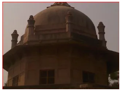
图2 .与热图像匹配后裁剪的可见图像

为了执行上述操作，基本上包含两张图像，一张参考图像和另一张要匹配的图像。 因此，下面的算法会找出参考图像的哪一部分出现在第二张图像中，并为您提供匹配图像部分的位置。

现在我们知道热图像中存在可见图像的哪一部分，我们可以裁剪可见图像，然后对生成的图像进行配准。

三、配准过程

为了执行配准，我们要做的是找出将像素从可见图像映射到热图像的特征点，这在本文中进行了解释，一旦我们获得了一定数量的像素，我们就会停止并开始映射这些像素，从而完成配准过程完成了。

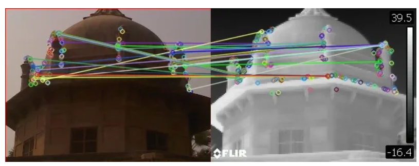
图3 热成像到可见光图像配准

一旦我们执行了配准，如果匹配正确，我们将获得具有配准图像的输出，如下图所示。

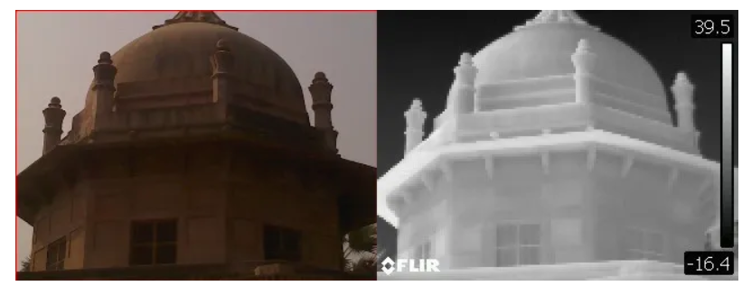
图4 最终输出结果

我对 400 张图像的数据集执行了此操作，获得的结果非常好。 错误数量很少，请参考下面的代码，看看一切是如何完成的。

 
from __future__ import print_function
import numpy as np
import argparse
import glob
import cv2
import os
 
MAX_FEATURES = 500
GOOD_MATCH_PERCENT = 0.15
 
#function to align the thermal and visible image, it returns the homography matrix 
def alignImages(im1, im2,filename):
 
  # Convert images to grayscale
  im1Gray = cv2.cvtColor(im1, cv2.COLOR_BGR2GRAY)
  im2Gray = cv2.cvtColor(im2, cv2.COLOR_BGR2GRAY)
   
  # Detect ORB features and compute descriptors.
  orb = cv2.ORB_create(MAX_FEATURES)
  keypoints1, descriptors1 = orb.detectAndCompute(im1Gray, None)
  keypoints2, descriptors2 = orb.detectAndCompute(im2Gray, None)
   
  # Match features.
  matcher = cv2.DescriptorMatcher_create(cv2.DESCRIPTOR_MATCHER_BRUTEFORCE_HAMMING)
  matches = matcher.match(descriptors1, descriptors2, None)
   
  # Sort matches by score
  matches.sort(key=lambda x: x.distance, reverse=False)
 
  # Remove not so good matches
  numGoodMatches = int(len(matches) * GOOD_MATCH_PERCENT)
  matches = matches[:numGoodMatches]
 
  # Draw top matches
  imMatches = cv2.drawMatches(im1, keypoints1, im2, keypoints2, matches, None)
  if os.path.exists(os.path.join(args["output"],"registration")):
    pass
  else:
   os.mkdir(os.path.join(args["output"],"registration"))
  cv2.imwrite(os.path.join(args["output"],"registration",filename), imMatches)
   
  # Extract location of good matches
  points1 = np.zeros((len(matches), 2), dtype=np.float32)
  points2 = np.zeros((len(matches), 2), dtype=np.float32)
 
  for i, match in enumerate(matches):
    points1[i, :] = keypoints1[match.queryIdx].pt
    points2[i, :] = keypoints2[match.trainIdx].pt
   
  # Find homography
  h, mask = cv2.findHomography(points1, points2, cv2.RANSAC)
 
  # Use homography
  height, width, channels = im2.shape
  im1Reg = cv2.warpPerspective(im1, h, (width, height))
   
  return im1Reg, h
 
# construct the argument parser and parse the arguments
# run the file with python registration.py --image filename
ap = argparse.ArgumentParser()
# ap.add_argument("-t", "--template", required=True, help="Path to template image")
ap.add_argument("-i", "--image", required=False,default=r"热红外图像的路径",
    help="Path to images where thermal template will be matched")
ap.add_argument("-v", "--visualize",required=False,default=r"真彩色影像的路径")
ap.add_argument("-o", "--output",required=False,default=r"保存路径")
args = vars(ap.parse_args())
 
# put the thermal image in a folder named thermal and the visible image in a folder named visible with the same name
# load the image image, convert it to grayscale, and detect edges
template = cv2.imread(args["image"])
template = cv2.cvtColor(template, cv2.COLOR_BGR2GRAY)
template = cv2.Canny(template, 50, 200)
(tH, tW) = template.shape[:2]
cv2.imshow("Template", template)
#cv2.waitKey(0)
 
# loop over the images to find the template in
 
# load the image, convert it to grayscale, and initialize the
# bookkeeping variable to keep track of the matched region
image = cv2.imread(args["visualize"])
gray = cv2.cvtColor(image, cv2.COLOR_BGR2GRAY)
found = None
 
# loop over the scales of the image
for scale in np.linspace(0.2, 1.0, 20)[::-1]:
    # resize the image according to the scale, and keep track
    # of the ratio of the resizing
    resized = cv2.resize(gray, (int(gray.shape[1] * scale),int(gray.shape[0] * scale)))
    r = gray.shape[1] / float(resized.shape[1])
 
    # if the resized image is smaller than the template, then break
    # from the loop
    if resized.shape[0] < tH or resized.shape[1] < tW:
        break
 
    # detect edges in the resized, grayscale image and apply template
    # matching to find the template in the image
    edged = cv2.Canny(resized, 50, 200)
    result = cv2.matchTemplate(edged, template, cv2.TM_CCOEFF)
    (_, maxVal, _, maxLoc) = cv2.minMaxLoc(result)
 
    # check to see if the iteration should be visualized
    if True:
        # draw a bounding box around the detected region
        clone = np.dstack([edged, edged, edged])
        cv2.rectangle(clone, (maxLoc[0], maxLoc[1]),
            (maxLoc[0] + tW, maxLoc[1] + tH), (0, 0, 255), 2)
        cv2.imshow("Visualize", clone)
        #cv2.waitKey(0)
 
    # if we have found a new maximum correlation value, then update
    # the bookkeeping variable
    if found is None or maxVal > found[0]:
        found = (maxVal, maxLoc, r)
 
# unpack the bookkeeping variable and compute the (x, y) coordinates
# of the bounding box based on the resized ratio
(_, maxLoc, r) = found
(startX, startY) = (int(maxLoc[0] * r), int(maxLoc[1] * r))
(endX, endY) = (int((maxLoc[0] + tW) * r), int((maxLoc[1] + tH) * r))
 
# draw a bounding box around the detected result and display the image
cv2.rectangle(image, (startX, startY), (endX, endY), (0, 0, 255), 2)
crop_img = image[startY:endY, startX:endX]
#cv2.imshow("Image", image)
cv2.imshow("Crop Image", crop_img)
#cv2.waitKey(0)
 
#name = r"E:\temp\data5/thermal/"+args["image"]+'.JPG'
thermal_image = cv2.imread(args["image"], cv2.IMREAD_COLOR)
 
#cropping out the matched part of the thermal image
crop_img = cv2.resize(crop_img, (thermal_image.shape[1], thermal_image.shape[0]))
 
#cropped image will be saved in a folder named output
if os.path.exists(os.path.join(args["output"],"process")):
   pass
else:
   os.mkdir(os.path.join(args["output"],"process"))
cv2.imwrite(os.path.join(args["output"],"process", os.path.basename(args["visualize"])),crop_img)
 
#both images are concatenated and saved in a folder named results
final = np.concatenate((crop_img, thermal_image), axis = 1)
if os.path.exists(os.path.join(args["output"],"results")):
   pass
else:
   os.mkdir(os.path.join(args["output"],"results"))
cv2.imwrite(os.path.join(args["output"],"results", os.path.basename(args["visualize"])),final)
 
#cv2.waitKey(0)
# Registration
# Read reference image
refFilename =  args["image"]
print("Reading reference image : ", refFilename)
imReference = cv2.imread(refFilename, cv2.IMREAD_COLOR)
 
# Read image to be aligned
imFilename = os.path.join(args["output"],"process", os.path.basename(args["visualize"]))
print("Reading image to align : ", imFilename);  
im = cv2.imread(imFilename, cv2.IMREAD_COLOR)
file_name=os.path.basename(args["image"])+'_registration.JPG'
imReg, h = alignImages(im,imReference,file_name)
cv2.imwrite(os.path.join(args["output"],"results", os.path.basename(args["image"])+'_result.JPG'),imReg)
print("Estimated homography : \n",  h)

我们已经成功地进行了热到可见图像配准。你可以用你的数据集来尝试一下，然后看看结果。

后续：

        因opencv版本问题做了修改，最终结果可以在registration和result保存路径下查看，其中opencv原因需要英文路径，调用使用方法如下：

python .\main.py -i “热红外影像路径” -v “真彩色影像路径” -o “保存路径”