
- 1【论文阅读】Hierarchical Multi-modal Contextual Attention Network for Fake News Detection --- 虚假新闻检测,多模态_多模态论文复现
- 2访问控制相关概念及常见模型_强制性访问控制也叫做基于什么的访问控制
- 3第三章:AI大模型的主要技术框架3.3 Hugging Face Transformers3.3.2 Transformers基本操作与实例
- 4微信小程序开发初学:超链接---navigator_微信开发者工具 超链接
- 5GPT系列解读--GPT1_gpt-1
- 6GPT语言模型:通过生成式预训练改善语言理解 OpenAI 2018_gpt模型中的生成过程是怎么样的?
- 7【Android FFMPEG 开发】FFMPEG 音视频同步 ( 音视频同步方案 | 视频帧 FPS 控制 | H.264 编码 I / P / B 帧 | PTS | 音视频同步 )_h26数据包修改fps
- 8计算机视觉-语义分割论文总结
- 9neo4j 大量数据的批量导入_neo4j批量处理数据
- 10Gartner发布2023年最新技术成熟度曲线,偶数科技位列湖仓一体代表厂商_2023 gartner magic quadrant for data lakehouse
Coursera自然语言处理专项课程03:Natural Language Processing with Sequence Models笔记 Week01
赞
踩
Natural Language Processing with Sequence Models
Course Certificate

本文是https://www.coursera.org/learn/sequence-models-in-nlp 这门课程的学习笔记,如有侵权,请联系删除。

文章目录
- Natural Language Processing with Sequence Models
- Week 01: Recurrent Neural Networks for Language Modeling
- Introduction to Neural Networks and TensorFlow
- Lab: Introduction to TensorFlow
- Practice Programming Assignment: Sentiment with Deep Neural Networks
- N-grams vs. Sequence Models
- Practice Quiz: RNNs for Language Modelling
- Programming Assignment: Deep N-grams
- 后记
Week 01: Recurrent Neural Networks for Language Modeling
Learn about the limitations of traditional language models and see how RNNs and GRUs use sequential data for text prediction. Then build your own next-word generator using a simple RNN on Shakespeare text data!
Learning Objectives
- Supervised machine learning
- Binary classification
- Neural networks
- N-grams
- Gated recurrent units
- Recurrent neural networks
Introduction to Neural Networks and TensorFlow
Neural Networks for Sentiment Analysis
Previously in the course you did sentiment analysis with logistic regression and naive Bayes. Those models were in a sense more naive, and are not able to catch the sentiment off a tweet like: "I am not happy " or “If only it was a good day”. When using a neural network to predict the sentiment of a sentence, you can use the following. Note that the image below has three outputs, in this case you might want to predict, “positive”, "neutral ", or “negative”.
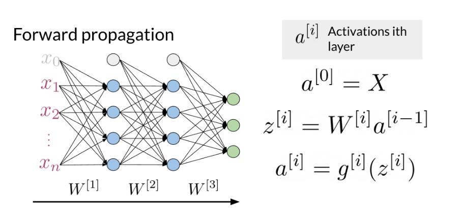
Note that the network above has three layers. To go from one layer to another you can use a W matrix to propagate to the next layer. Hence, we call this concept of going from the input until the final layer, forward propagation. To represent a tweet, you can use the following:
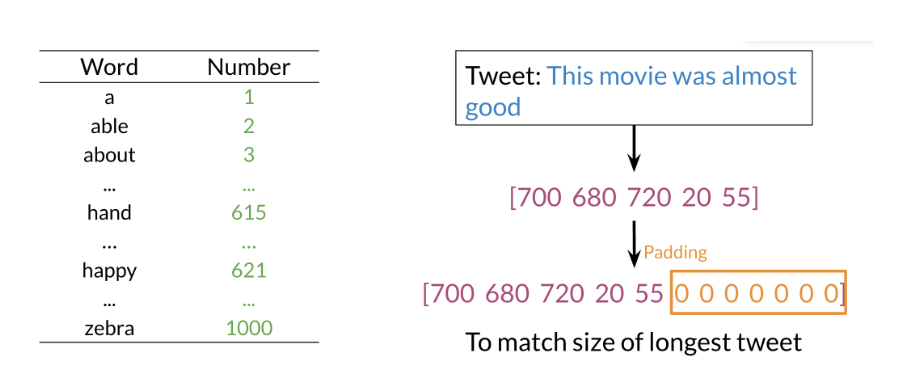
Note, that we add zeros for padding to match the size of the longest tweet.
A neural network in the setup you can see above can only process one such tweet at a time. In order to make training more efficient (faster) you want to process many tweets in parallel. You achieve this by putting many tweets together into a matrix and then passing this matrix (rather than individual tweets) through the neural network. Then the neural network can perform its computations on all tweets at the same time.
Dense Layers and ReLU
The Dense layer is the computation of the inner product between a set of trainable weights (weight matrix) and an input vector. The visualization of the dense layer can be seen in the image below.
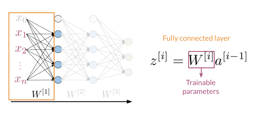
The orange box in the image above shows the dense layer. An activation layer is the set of blue nodes shown with the orange box in the image below. Concretely one of the most commonly used activation layers is the rectified linear unit (ReLU).
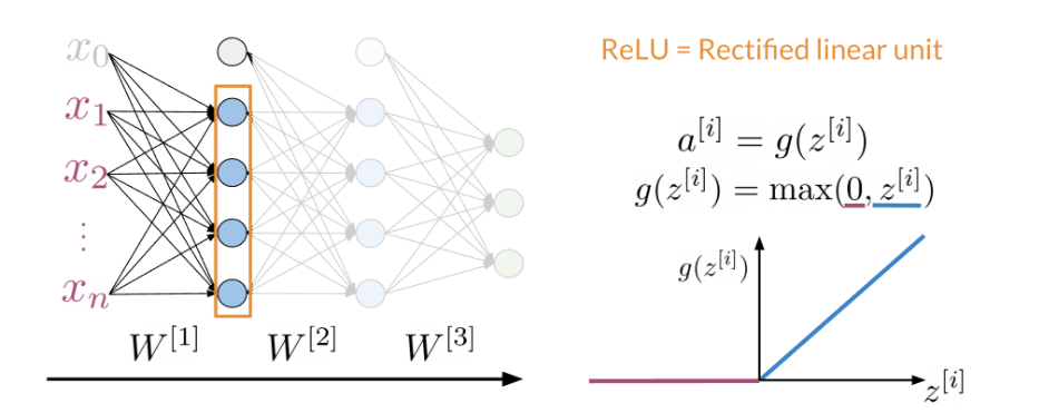
ReLU(x) is defined as max(0,x) for any input x.
Embedding and Mean Layers
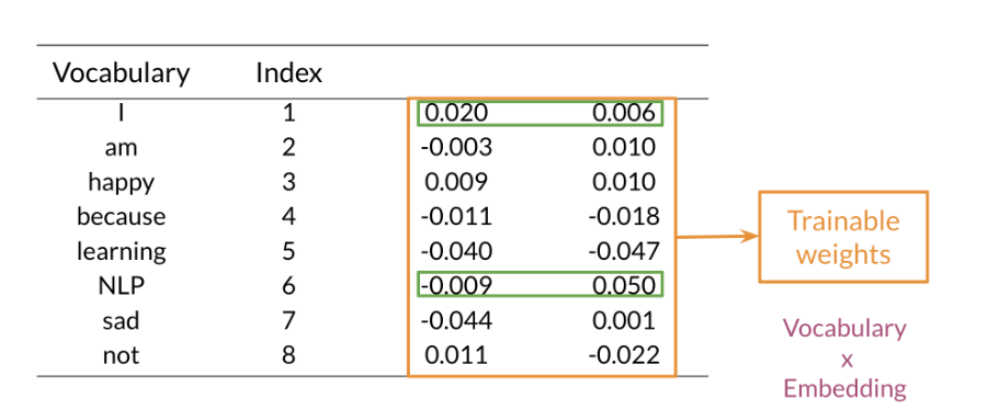
Using an embedding layer you can learn word embeddings for each word in your vocabulary as follows:
The mean layer allows you to take the average of the embeddings. You can visualize it as follows:
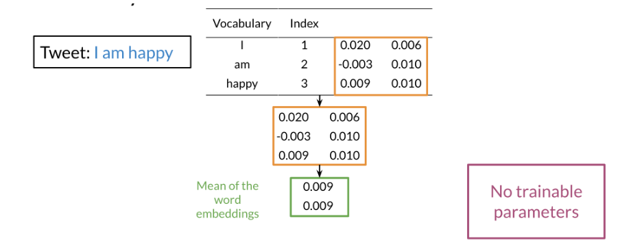
This layer does not have any trainable parameters.
Lab: Introduction to TensorFlow
Lab 1: TensorFlow Tutorial and Some Useful Functions
Welcome to the first lab in this course. Here you will see and try out some basics of TensorFlow and get familiar with some of the useful functions that you will use across the assignments. If you already know TensorFlow well, feel free to skip this notebook.
For the demonstration purposes you will use the IMDB reviews dataset, on which you will perform sentiment classification. The dataset consists of 50,000 movie reviews from the Internet Movie Database (IMDB), but has been shrinked down to 6,000 reviews to save space and ensure faster performance of the notebook.
A part of the code in this notebook is reused from the TensorFlow official tutorial.
1. Import the libraries
# To silence the TensorFlow warnings, you can use the following code before you import the TensorFlow library.
import os
os.environ['TF_CPP_MIN_LOG_LEVEL'] = '3'

import numpy as np
import tensorflow as tf
from tensorflow.keras.preprocessing.text import Tokenizer
from tensorflow.keras import layers
from tensorflow.keras import losses
import re
import string
import matplotlib.pyplot as plt

print("Imports successful!")
- 1
- 2
- 3
- 4
- 5
- 6
- 7
- 8
- 9
- 10
- 11
- 12
- 13
- 14
Setting the random seed allows you to have control over the (pseudo)random numbers. When you are working with neural networks this is a good idea, so you can get reproducible results (when you run the calculation twice you will always get the same “random” numbers). It is especially important not to mess with the random seed in your assignments, as they are used for checking whether your values are set correctly.
# Select your favourite number for the random seed
seed = 42

# Sets the global random seed for numpy.
np.random.seed(seed)
# Sets the global random seed for TensorFlow.
tf.random.set_seed(seed)

print(f"Random seed set to {seed}")
- 1
- 2
- 3
- 4
- 5
- 6
- 7
- 8
- 9
Output
Random seed set to 42
- 1
2. Load the data
First you set the path to the directory where you store your data.
data_dir = './data/aclImdb'
- 1
Below, you will use the function tf.keras.utils.text_dataset_from_directory, that generates a tf.data.Dataset from text files in a directory.
TensorFlow allows you for very easy dataset creation, provided that you have data in the following folder substructure.
main_directory/
... class_a/
...... a_text_1.txt
...... a_text_2.txt
... class_b/
...... b_text_1.txt
...... b_text_2.txt
- 1
- 2
- 3
- 4
- 5
- 6
- 7
Calling text_dataset_from_directory(...) will return a tf.data.Dataset that yields batches of texts from the subdirectories class_a and class_b, together with labels 0 and 1 (0 corresponding to class_a and 1 corresponding to class_b).
Only .txt files are supported at this time, but there are equivalent functions for different kinds of data, for example image_dataset_from_directory for images.
In your case you have two main directories: ./data/aclImdb/train/ and ./data/aclImdb/test/. Within both of these two directories you have data separated in two classes: neg and pos. So your actual folder structure looks like this:
./data/aclImdb/train/
... neg/
...... text_1.txt
...... text_2.txt
...... ...
... pos/
...... text_1.txt
...... text_2.txt
...... ...
- 1
- 2
- 3
- 4
- 5
- 6
- 7
- 8
- 9
And the same for the test folder, with many .txt files in each subfolder.
You can explore the folders by clicking File and then Open in the menu above, or by clicking on the Jupyter symbol.
In the cell below, you will load the data. Note the different parameters that you can use when loading the data. For example: originally you only have the data split only to training and test sets, but you can very easily split the datasets further, by using just a few parameters.
# Here you have two main directories: one for train and one for test data.
# You load files from each to create training and test datasets.

# Create the training set. Use 80% of the data and keep the remaining 20% for the validation.
raw_training_set = tf.keras.utils.text_dataset_from_directory(
    f'{data_dir}/train',
    labels='inferred',
    label_mode='int',
    batch_size=32,
    validation_split=0.2,
    subset='training',
    seed=seed
)

# Create the validation set. Use 20% of the data that was not used for training.
raw_validation_set = tf.keras.utils.text_dataset_from_directory(
    f'{data_dir}/train',
    labels='inferred',
    label_mode='int',
    batch_size=32,
    validation_split=0.2,
    subset='validation',
    seed=seed
)

# Create the test set.
raw_test_set = tf.keras.utils.text_dataset_from_directory(
    f'{data_dir}/test',
    labels='inferred',
    label_mode='int',
    batch_size=32,
)

- 1
- 2
- 3
- 4
- 5
- 6
- 7
- 8
- 9
- 10
- 11
- 12
- 13
- 14
- 15
- 16
- 17
- 18
- 19
- 20
- 21
- 22
- 23
- 24
- 25
- 26
- 27
- 28
- 29
- 30
- 31
- 32
Output
Found 5000 files belonging to 2 classes.
Using 4000 files for training.
Found 5000 files belonging to 2 classes.
Using 1000 files for validation.
Found 5000 files belonging to 2 classes.
- 1
- 2
- 3
- 4
- 5
Check that the labels 0 and 1 correctly correspond to the negative and positive examples respectively.
print(f"Label 0 corresponds to {raw_training_set.class_names[0]}")
print(f"Label 1 corresponds to {raw_training_set.class_names[1]}")
- 1
- 2
Output
Label 0 corresponds to neg
Label 1 corresponds to pos
- 1
- 2
If you want to look at a small subset of your dataset, you can use .take() method, by passing it the count parameter. The method returns a new dataset of the size at most count, where count is the number of batches. You can read more about tf.data.Dataset and the take method here.
# Take one batch from the dataset and print out the first three datapoints in the batch
for text_batch, label_batch in raw_training_set.take(1):
    for i in range(3):
        print(f"Review:\n {text_batch.numpy()[i]}")
        print(f"Label: {label_batch.numpy()[i]}\n")
- 1
- 2
- 3
- 4
- 5
Output
Review:
 b'This is a reunion, a team, and a great episode of Justice. From hesitation to resolution, Clark has made a important leap from a troubled teenager who was afraid of a controlled destiny, to a Superman who, like Green Arrow, sets aside his emotions to his few loved ones, ready to save the whole planet. This is not just a thrilling story about teamwork, loyalty, and friendship; this is also about deciding what\'s more important in life, a lesson for Clark. I do not want the series to end, but I hope the ensuing episodes will strictly stick to what Justice shows without any "rewind" pushes and put a good end here of Smallville---and a wonderful beginning of Superman.<br /><br />In this episode, however, we should have seen more contrast between Lex and the Team. Nine stars should give it enough credit.'
Label: 1

Review:
 b'"Hey Babu Riba" is a film about a young woman, Mariana (nicknamed "Esther" after a famous American movie star), and four young men, Glenn, Sacha, Kicha, and Pop, all perhaps 15-17 years old in 1953 Belgrade, Yugoslavia. The five are committed friends and crazy about jazz, blue jeans, or anything American it seems.<br /><br />The very close relationship of the teenagers is poignant, and ultimately a sacrifice is willingly made to try to help one of the group who has fallen on unexpected difficulties. In the wake of changing communist politics, they go their separate ways and reunite in 1985 (the year before the film was made).<br /><br />I enjoyed the film with some reservations. The subtitles for one thing were difficult. Especially in the beginning, there were a number of dialogues which had no subtitles at all. Perhaps the conversational pace required it, but I couldn\'t always both read the text and absorb the scene, which caused me to not always understand which character was involved. I watched the movie (a video from our public library) with a friend, and neither of us really understood part of the story about acquiring streptomycin for a sick relative.<br /><br />This Yugoslavian coming of age film effectively conveyed the teenagers\' sense of invulnerability, idealism, and strong and loyal bonds to each other. There is a main flashforward, and it was intriguing, keeping me guessing until the end as to who these characters were vis-a-vis the 1953 cast, and what had actually happened.<br /><br />I would rate it 7 out of 10, and would like to see other films by the director, Jovan Acin (1941-1991).'
Label: 1

Review:
 b"No message. No symbolism. No dark undercurrents.Just a wonderful melange of music, nostalgia and good fun put to-gether by people who obviously had a great time doing it. It's a refreshing antidote to some of the pretentious garbage being ground out by the studios. Of course ANYTHING with the incomparable Judi Dench is worth watching. And Cleo Laine's brilliant jazz singing is a bonus. This lady is in the same league as the late Ella. This goes on my movie shelf to be pulled out again anytime I feel the need for a warm experience and a hearty good natured chuckle. Just a wonderful film!"
Label: 1
- 1
- 2
- 3
- 4
- 5
- 6
- 7
- 8
- 9
- 10
- 11
3. Prepare the Data
Now that you have seen how the dataset looks like, you need to prepare it in the format that a neural network understands. For this, you will use the tf.keras.layers.TextVectorization layer.
This layer converts text to vectors that can then be fed to a neural network. A very useful feature is that you can pass it another function that performs custom standardization of text. This includes lowercasing the text, removing punctuation and/or HTML elements, web links or certain tags. This is very important, as every dataset requires different standardization, depending on its contents. After the standardization, the layer tokenizes the text (splits into words) and vectorizes it (converts from words to numbers) so that it can be fed to the neural network. The output_sequence_length is set to 250, which means that the layer will pad shorter sequences or truncate longer sequences, so they will al have the same length. This is done so that all the inout vectors are the same length and can be nicely put together into matrices.
# Set the maximum number of words
max_features = 10000

# Define the custom standardization function
def custom_standardization(input_data):
    # Convert all text to lowercase
    lowercase = tf.strings.lower(input_data)
    # Remove HTML tags
    stripped_html = tf.strings.regex_replace(lowercase, '<br />', ' ')
    # Remove punctuation
    replaced = tf.strings.regex_replace(
        stripped_html,
        '[%s]' % re.escape(string.punctuation),
        ''
    )
    return replaced

# Create a layer that you can use to convert text to vectors
vectorize_layer = layers.TextVectorization(
    standardize=custom_standardization,
    max_tokens=max_features,
    output_mode='int',
    output_sequence_length=250)
- 1
- 2
- 3
- 4
- 5
- 6
- 7
- 8
- 9
- 10
- 11
- 12
- 13
- 14
- 15
- 16
- 17
- 18
- 19
- 20
- 21
- 22
- 23
Next, you call adapt to fit the state of the preprocessing layer to the dataset. This will cause the model to build a vocabulary (an index of strings to integers). If you want to access the vocabulary, you can call the .get_vocabulary() on the layer.
# Build the vocabulary
train_text = raw_training_set.map(lambda x, y: x)
vectorize_layer.adapt(train_text)

# Print out the vocabulary size
print(f"Vocabulary size: {len(vectorize_layer.get_vocabulary())}")
- 1
- 2
- 3
- 4
- 5
- 6
raw_training_set.map(lambda x, y: x)解释:
这行代码使用了 TensorFlow 的 map 函数,它将函数应用于数据集中的每个元素。在这里,raw_training_set 是一个数据集,每个元素都是一个 (x, y) 元组,其中 x 是文本数据,y 是对应的标签。Lambda 函数 lambda x, y: x 用于提取每个元组中的文本数据 x,并将其作为输出。因此,train_text 包含了所有训练集中的文本数据。
Output
Vocabulary size: 10000
- 1
Now you can define the final function that you will use to vectorize the text and see what it looks like.
Note that you need to add the .expand_dims(). This adds another dimension to your data and is very commonly used when processing data to add an additional dimension to accomodate for the batches.
# Define the final function that you will use to vectorize the text.
def vectorize_text(text, label):
    text = tf.expand_dims(text, -1)
    return vectorize_layer(text), label

# Get one batch and select the first datapoint
text_batch, label_batch = next(iter(raw_training_set))
first_review, first_label = text_batch[0], label_batch[0]

# Show the raw data
print(f"Review:\n{first_review}")
print(f"\nLabel: {raw_training_set.class_names[first_label]}")
# Show the vectorized data
print(f"\nVectorized review\n{vectorize_text(first_review, first_label)}")
- 1
- 2
- 3
- 4
- 5
- 6
- 7
- 8
- 9
- 10
- 11
- 12
- 13
- 14
Output
Review:
b"Okay, so the plot is on shaky ground. Yeah, all right, so there are some randomly inserted song and/or dance sequences (for example: Adam's concert and Henri's stage act). And Leslie Caron can't really, um, you know... act.<br /><br />But somehow, 'An American In Paris' manages to come through it all as a polished, first-rate musical--largely on the basis of Gene Kelly's incredible dancing talent and choreography, and the truckloads of charm he seems to be importing into each scene with Caron. (He needs to, because she seems to have a... problem with emoting.) <br /><br />The most accomplished and technically awe-inspiring number in this musical is obviously the 16-minute ballet towards the end of the film. It's stunningly filmed, and Kelly and Caron dance beautifully. But my favourite number would have to be Kelly's character singing 'I Got Rhythm' with a bunch of French school-children, then breaking into an array of American dances. It just goes to prove how you don't need special effects when you've got some real *talent*.<br /><br />Not on the 'classics' level with 'Singin' In The Rain', but pretty high up there nonetheless. Worth the watch!"

Label: pos

Vectorized review
(<tf.Tensor: shape=(1, 250), dtype=int64, numpy=
array([[ 947,   38,    2,  112,    7,   20, 6022, 1754, 1438,   31,  201,
          38,   46,   24,   47, 6565, 8919,  603, 2928,  831,  858,   15,
         476, 3241, 3010,    4,    1,  892,  478,    4, 3553, 5885,  175,
          63, 6992,   21,  118,  478,   18,  813,   33,  329,    8, 1466,
        1029,    6,  227,  143,    9,   31,   14,    3, 6590, 9055,    1,
          20,    2, 3025,    5, 1996,    1, 1085,  914,  597,    4, 2733,
           4,    2,    1,    5, 1411,   27,  190,    6,   26,    1,   77,
         244,  130,   16, 5885,   27,  731,    6,   80,   53,  190,    6,
          25,    3,  425,   16,    1,    2,   85, 3622,    4, 2603,    1,
         593,    8,   10,  663,    7,  506,    2,    1, 4342, 1089,    2,
         121,    5,    2,   19,   29, 5994,  886,    4, 1561,    4, 5885,
         831, 1415,   18,   55, 1496,  593,   62,   25,    6,   26,    1,
         105,  965,   11,  186, 4687,   16,    3,  862,    5, 1001,    1,
          96, 2442,   77,   33, 7537,    5,  329, 4825,    9,   41,  264,
           6, 2131,   86,   21,   87,  333,  290,  317,   51,  699,  186,
          47,  144,  597,   23,   20,    2, 2008,  557,   16, 7714,    8,
           2, 2477,   18,  179,  307,   57,   46, 2878,  268,    2,  106,
           0,    0,    0,    0,    0,    0,    0,    0,    0,    0,    0,
           0,    0,    0,    0,    0,    0,    0,    0,    0,    0,    0,
           0,    0,    0,    0,    0,    0,    0,    0,    0,    0,    0,
           0,    0,    0,    0,    0,    0,    0,    0,    0,    0,    0,
           0,    0,    0,    0,    0,    0,    0,    0,    0,    0,    0,
           0,    0,    0,    0,    0,    0,    0,    0]])>, <tf.Tensor: shape=(), dtype=int32, numpy=1>)
- 1
- 2
- 3
- 4
- 5
- 6
- 7
- 8
- 9
- 10
- 11
- 12
- 13
- 14
- 15
- 16
- 17
- 18
- 19
- 20
- 21
- 22
- 23
- 24
- 25
- 26
- 27
- 28
- 29
- 30
Now you can apply the vectorization function to vectorize all three datasets.
train_ds = raw_training_set.map(vectorize_text)
val_ds = raw_validation_set.map(vectorize_text)
test_ds = raw_test_set.map(vectorize_text)
- 1
- 2
- 3
在 TensorFlow 中,map 方法用于对数据集中的每个样本应用一个函数。
Configure the Dataset
There are two important methods that you should use when loading data to make sure that I/O does not become blocking.
.cache() keeps data in memory after it’s loaded off disk. This will ensure the dataset does not become a bottleneck while training your model. If your dataset is too large to fit into memory, you can also use this method to create a performant on-disk cache, which is more efficient to read than many small files.
.prefetch() overlaps data preprocessing and model execution while training.
You can learn more about both methods, as well as how to cache data to disk in the data performance guide.
For very interested, you can read more about tf.data and AUTOTUNE in this paper, but be aware that this is already very advanced information about how TensorFlow works.
AUTOTUNE = tf.data.AUTOTUNE

train_ds = train_ds.cache().prefetch(buffer_size=AUTOTUNE)
test_ds = test_ds.cache().prefetch(buffer_size=AUTOTUNE)
- 1
- 2
- 3
- 4
在这段代码中,AUTOTUNE 是一个特殊的值,用于告诉 TensorFlow 在运行时根据可用的计算资源自动选择合适的参数值。tf.data.AUTOTUNE 的值在不同的硬件和工作负载下可能会有所不同,它会根据系统资源(如 CPU 和内存)的状况来自动调整参数。
在这里,cache() 方法将数据集缓存起来,以提高数据加载的效率。缓存数据集可以确保数据在被重复使用时不会重新加载,从而节省了加载时间。
prefetch() 方法用于在训练过程中异步加载数据,以减少训练时的等待时间。buffer_size 参数指定了要预取的样本数。通过调用 prefetch(buffer_size=AUTOTUNE),我们告诉 TensorFlow 在运行时自动选择合适的预取数量,以优化数据加载的性能。
4. Create a Sequential Model
A Sequential model is appropriate for a simple stack of layers where each layer has exactly one input tensor and one output tensor (layers follow each other in a sequence and there are no additional connections).
Here you will use a Sequential model using only three layers:
- An Embedding layer. This layer takes the integer-encoded reviews and looks up an embedding vector for each word-index. These vectors are learned as the model trains. The vectors add a dimension to the output array. The resulting dimensions are: (batch, sequence, embedding).
- A GlobalAveragePooling1D layer returns a fixed-length output vector for each example by averaging over the sequence dimension. This allows the model to handle input of variable length, in the simplest way possible.
- A Dense layer with a single output node.
embedding_dim = 16

# Create the model by calling tf.keras.Sequential, where the layers are given in a list.
model_sequential = tf.keras.Sequential([
    layers.Embedding(max_features, embedding_dim),
    layers.GlobalAveragePooling1D(),
    layers.Dense(1, activation='sigmoid')
])

# Print out the summary of the model
model_sequential.summary()
- 1
- 2
- 3
- 4
- 5
- 6
- 7
- 8
- 9
- 10
- 11
这段代码使用了 tf.keras.Sequential 来创建一个序列模型,其中包含了几个层:
-
layers.Embedding(max_features, embedding_dim):这是一个嵌入层,用于将输入的整数序列(每个整数代表一个单词的索引)转换为密集的向量表示。max_features表示词汇表的大小,embedding_dim表示嵌入向量的维度。 -
layers.GlobalAveragePooling1D():这是一个全局平均池化层,用于在时间维度上对输入的一维特征序列进行平均池化,得到一个全局的特征表示。 -
layers.Dense(1, activation='sigmoid'):这是一个全连接层,包含一个神经元,使用 Sigmoid 激活函数。这个层用于将全局池化得到的特征表示映射到一个输出值,通常用于二分类任务。
这个序列模型按照给定的顺序依次堆叠这些层,构建了一个端到端的深度学习模型,用于处理文本数据并执行二分类任务。
Output
Model: "sequential"
_________________________________________________________________
 Layer (type)                Output Shape              Param #
=================================================================
 embedding (Embedding)       (None, None, 16)          160000

 global_average_pooling1d (  (None, 16)                0
 GlobalAveragePooling1D)

 dense (Dense)               (None, 1)                 17

=================================================================
Total params: 160017 (625.07 KB)
Trainable params: 160017 (625.07 KB)
Non-trainable params: 0 (0.00 Byte)
_________________________________________________________________
- 1
- 2
- 3
- 4
- 5
- 6
- 7
- 8
- 9
- 10
- 11
- 12
- 13
- 14
- 15
- 16
Compile the model. Choose the loss function, the optimizer and any additional metrics you want to calculate. Since this is a binary classification problem you can use the losses.BinaryCrossentropy loss function.
model_sequential.compile(loss=losses.BinaryCrossentropy(),
              optimizer='adam',
              metrics=['accuracy'])
- 1
- 2
- 3
5. Create a Model Using Functional API
You can use the functional API when you want to create more complex models, but it works just as well for the simple models like the one above. The functional API can handle models with non-linear topology, shared layers, and even multiple inputs or outputs.
The biggest difference at the first glance is that you need to explicitly state the input. Then you use the layers as functions and pass previous layers as parameters into the functions. In the end you build a model, where you pass it the input and the output of the neural network. All of the information from between them (hidden layers) is already hidden in the output layer (remember how each layer takes the previous layer in as a parameter).
# Define the inputs
inputs = tf.keras.Input(shape=(None,))

# Define the first layer
embedding = layers.Embedding(max_features, embedding_dim)
# Call the first layer with inputs as the parameter
x = embedding(inputs)

# Define the second layer
pooling = layers.GlobalAveragePooling1D()
# Call the first layer with the output of the previous layer as the parameter
x = pooling(x)

# Define and call in the same line. (Same thing used two lines of code above
# for other layers. You can use any option you prefer.)
outputs = layers.Dense(1, activation='sigmoid')(x)
#The two-line alternative to the one layer would be:
# dense = layers.Dense(1, activation='sigmoid')
# x = dense(x)


# Create the model
model_functional = tf.keras.Model(inputs=inputs, outputs=outputs)

# Print out the summary of the model
model_functional.summary()
- 1
- 2
- 3
- 4
- 5
- 6
- 7
- 8
- 9
- 10
- 11
- 12
- 13
- 14
- 15
- 16
- 17
- 18
- 19
- 20
- 21
- 22
- 23
- 24
- 25
- 26
Output
Model: "model"
_________________________________________________________________
 Layer (type)                Output Shape              Param #
=================================================================
 input_1 (InputLayer)        [(None, None)]            0

 embedding_1 (Embedding)     (None, None, 16)          160000

 global_average_pooling1d_1  (None, 16)                0
  (GlobalAveragePooling1D)

 dense_1 (Dense)             (None, 1)                 17

=================================================================
Total params: 160017 (625.07 KB)
Trainable params: 160017 (625.07 KB)
Non-trainable params: 0 (0.00 Byte)
_________________________________________________________________
- 1
- 2
- 3
- 4
- 5
- 6
- 7
- 8
- 9
- 10
- 11
- 12
- 13
- 14
- 15
- 16
- 17
- 18
这个输出的形状描述显示了每个层的输出形状,但不包括批量大小(Batch Size)。在这个例子中,(None, None, 16) 表示第一个维度是批量大小(Batch Size),第二个维度是序列长度(Sequence Length),第三个维度是特征维度(Feature Dimension)。
具体来说:
(None, None)表示输入层(Input Layer)接受的是二维张量,第一个维度为批量大小,第二个维度为序列长度。None表示这两个维度的长度可以是任意值,这取决于输入数据的实际形状。(None, None, 16)表示嵌入层(Embedding Layer)的输出是一个三维张量,第一个维度为批量大小,第二个维度为序列长度,第三个维度为特征维度。在这个例子中,特征维度为16。(None, 16)表示全局平均池化层(Global Average Pooling 1D Layer)的输出是一个二维张量,第一个维度为批量大小,第二个维度为特征维度。在这个例子中,特征维度为16。(None, 1)表示密集连接层(Dense Layer)的输出是一个二维张量,第一个维度为批量大小,第二个维度为神经元数量。在这个例子中,有一个神经元,因此输出的维度为(None, 1)。
因此,这里给出的是每个层的输出形状,而不是输出维度。
Compile the model: choose the loss, optimizer and any additional metrics you want to calculate. This is the same as for the sequential model.
model_functional.compile(loss=losses.BinaryCrossentropy(),
              optimizer='adam',
              metrics=['accuracy'])
- 1
- 2
- 3
6. Train the Model
Above, you have defined two different models: one with a functional api and one sequential model. From now on, you will use only one of them. feel free to change which model you want to use in the next cell. The results should be the same, as the architectures of both models are the same.
# Select which model you want to use and train. the results should be the same
model = model_functional # model = model_sequential
- 1
- 2
Now you will train the model. You will pass it the training and validation dataset, so it can compute the accuracy metric on both during training.
epochs = 25
history = model.fit(
    train_ds,
    validation_data=val_ds,
    epochs=epochs,
    verbose=2
)
- 1
- 2
- 3
- 4
- 5
- 6
- 7
Output
Epoch 1/25
125/125 - 2s - loss: 0.6903 - accuracy: 0.5648 - val_loss: 0.6864 - val_accuracy: 0.6810 - 2s/epoch - 15ms/step
Epoch 2/25
125/125 - 1s - loss: 0.6788 - accuracy: 0.7032 - val_loss: 0.6723 - val_accuracy: 0.7200 - 765ms/epoch - 6ms/step
Epoch 3/25
125/125 - 1s - loss: 0.6582 - accuracy: 0.7460 - val_loss: 0.6501 - val_accuracy: 0.7420 - 769ms/epoch - 6ms/step
Epoch 4/25
125/125 - 1s - loss: 0.6295 - accuracy: 0.7753 - val_loss: 0.6224 - val_accuracy: 0.7680 - 658ms/epoch - 5ms/step
Epoch 5/25
125/125 - 1s - loss: 0.5958 - accuracy: 0.7920 - val_loss: 0.5931 - val_accuracy: 0.7860 - 644ms/epoch - 5ms/step
Epoch 6/25
125/125 - 1s - loss: 0.5604 - accuracy: 0.8102 - val_loss: 0.5645 - val_accuracy: 0.7980 - 649ms/epoch - 5ms/step
Epoch 7/25
125/125 - 1s - loss: 0.5251 - accuracy: 0.8335 - val_loss: 0.5377 - val_accuracy: 0.8020 - 659ms/epoch - 5ms/step
Epoch 8/25
125/125 - 1s - loss: 0.4912 - accuracy: 0.8530 - val_loss: 0.5129 - val_accuracy: 0.8070 - 640ms/epoch - 5ms/step
Epoch 9/25
125/125 - 1s - loss: 0.4592 - accuracy: 0.8712 - val_loss: 0.4905 - val_accuracy: 0.8190 - 784ms/epoch - 6ms/step
Epoch 10/25
125/125 - 1s - loss: 0.4294 - accuracy: 0.8832 - val_loss: 0.4703 - val_accuracy: 0.8260 - 695ms/epoch - 6ms/step
Epoch 11/25
125/125 - 1s - loss: 0.4020 - accuracy: 0.8932 - val_loss: 0.4524 - val_accuracy: 0.8330 - 633ms/epoch - 5ms/step
Epoch 12/25
125/125 - 1s - loss: 0.3769 - accuracy: 0.9025 - val_loss: 0.4366 - val_accuracy: 0.8430 - 659ms/epoch - 5ms/step
Epoch 13/25
125/125 - 1s - loss: 0.3540 - accuracy: 0.9065 - val_loss: 0.4227 - val_accuracy: 0.8470 - 609ms/epoch - 5ms/step
Epoch 14/25
125/125 - 1s - loss: 0.3331 - accuracy: 0.9143 - val_loss: 0.4105 - val_accuracy: 0.8490 - 620ms/epoch - 5ms/step
Epoch 15/25
125/125 - 1s - loss: 0.3140 - accuracy: 0.9233 - val_loss: 0.3998 - val_accuracy: 0.8580 - 624ms/epoch - 5ms/step
Epoch 16/25
125/125 - 1s - loss: 0.2965 - accuracy: 0.9293 - val_loss: 0.3903 - val_accuracy: 0.8560 - 655ms/epoch - 5ms/step
Epoch 17/25
125/125 - 1s - loss: 0.2804 - accuracy: 0.9327 - val_loss: 0.3820 - val_accuracy: 0.8560 - 673ms/epoch - 5ms/step
Epoch 18/25
125/125 - 1s - loss: 0.2654 - accuracy: 0.9377 - val_loss: 0.3747 - val_accuracy: 0.8560 - 718ms/epoch - 6ms/step
Epoch 19/25
125/125 - 1s - loss: 0.2515 - accuracy: 0.9427 - val_loss: 0.3683 - val_accuracy: 0.8580 - 659ms/epoch - 5ms/step
Epoch 20/25
125/125 - 1s - loss: 0.2385 - accuracy: 0.9467 - val_loss: 0.3626 - val_accuracy: 0.8630 - 632ms/epoch - 5ms/step
Epoch 21/25
125/125 - 1s - loss: 0.2263 - accuracy: 0.9513 - val_loss: 0.3576 - val_accuracy: 0.8630 - 644ms/epoch - 5ms/step
Epoch 22/25
125/125 - 1s - loss: 0.2149 - accuracy: 0.9540 - val_loss: 0.3531 - val_accuracy: 0.8620 - 649ms/epoch - 5ms/step
Epoch 23/25
125/125 - 1s - loss: 0.2041 - accuracy: 0.9582 - val_loss: 0.3492 - val_accuracy: 0.8630 - 657ms/epoch - 5ms/step
Epoch 24/25
125/125 - 1s - loss: 0.1939 - accuracy: 0.9622 - val_loss: 0.3458 - val_accuracy: 0.8630 - 682ms/epoch - 5ms/step
Epoch 25/25
125/125 - 1s - loss: 0.1842 - accuracy: 0.9643 - val_loss: 0.3428 - val_accuracy: 0.8620 - 832ms/epoch - 7ms/step
- 1
- 2
- 3
- 4
- 5
- 6
- 7
- 8
- 9
- 10
- 11
- 12
- 13
- 14
- 15
- 16
- 17
- 18
- 19
- 20
- 21
- 22
- 23
- 24
- 25
- 26
- 27
- 28
- 29
- 30
- 31
- 32
- 33
- 34
- 35
- 36
- 37
- 38
- 39
- 40
- 41
- 42
- 43
- 44
- 45
- 46
- 47
- 48
- 49
- 50
Now you can use model.evaluate() to evaluate the model on the test dataset.
loss, accuracy = model.evaluate(test_ds)

print(f"Loss: {loss}")
print(f"Accuracy: {accuracy}")
- 1
- 2
- 3
- 4
Output
157/157 [==============================] - 1s 8ms/step - loss: 0.3642 - accuracy: 0.8452
Loss: 0.36415866017341614
Accuracy: 0.8452000021934509
- 1
- 2
- 3
When you trained the model, you saved the history in the history variable. Here you can access a dictionary that contains everything that happened during the training. In your case it saves the losses and the accuracy on both training and validation sets. You can plot it to gain some insights into how the training is progressing.
def plot_metrics(history, metric):
    plt.plot(history.history[metric])
    plt.plot(history.history[f'val_{metric}'])
    plt.xlabel("Epochs")
    plt.ylabel(metric.title())
    plt.legend([metric, f'val_{metric}'])
    plt.show()

plot_metrics(history, "accuracy")
plot_metrics(history, "loss")
- 1
- 2
- 3
- 4
- 5
- 6
- 7
- 8
- 9
- 10
Output
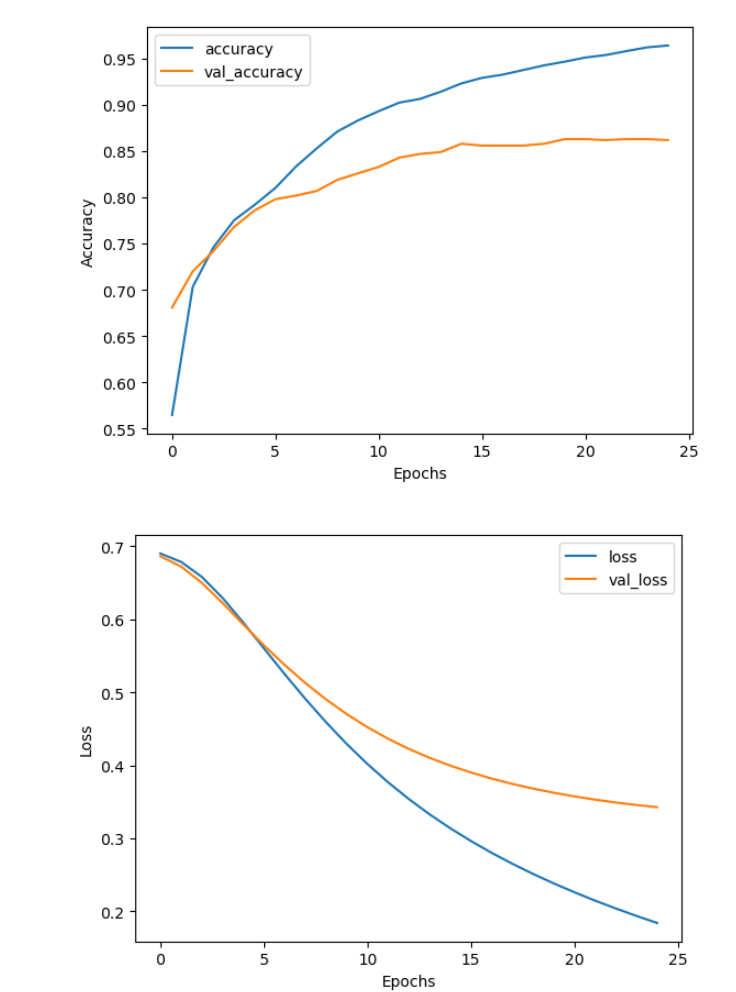
You can see that after 25 epochs, the training accuracy still goes up, but the validation accuracy already plateaus at around 86%. On the other hand both training and validation losses are still decreasing, which means that while the model does not learn to predict more cases accurately, it still gets more confident in its predictions. Here you used the simplest possible model: you have used embeddings, averaging layer and a dense layer with one output. You can try different architectures to see if the model improves. Perhaps you can add some dropout layers to reduce the chance of overfitting, or you can try a completely different architecture, like using convolutional layers or reccurent layers. You will learn a lot more about recurrent neural networks in the later weeks of this course.
7. Predict on Your Own Data
Finally, you can use the model to predict on any new data you may have. You can use it to predict the sentiment of examples in the test dataset (which the model has not seen in the training process) or use some completely new examples.
Here you will expand your model to be able to predict on raw strings (rather than on vectorized examples). Previously, you applied the TextVectorization layer to the dataset before feeding it to the model. To simplify deploying the model, you can include the TextVectorization layer inside your model and then predict on raw strings. To do so, you can create a new sequential model where you merge the vectorization layer with your trained model using the weights you just trained.
# Make a new sequential model using the vectorization layer and the model you just trained.
export_model = tf.keras.Sequential([
  vectorize_layer,
  model]
)

# Compile the model
export_model.compile(
    loss=losses.BinaryCrossentropy(from_logits=False), optimizer="adam", metrics=['accuracy']
)
- 1
- 2
- 3
- 4
- 5
- 6
- 7
- 8
- 9
- 10
Now you can use this model to predict on some of your own examples. You can do it simply by calling model.predict()
examples = ['this movie was very, very good', 'quite ok', 'the movie was not bad', 'bad', 'negative disappointed bad scary', 'this movie was stupid']

results = export_model.predict(examples, verbose=False)

for result, example in zip(results, examples):
    print(f'Result: {result[0]:.3f},   Label: {int(np.round(result[0]))},   Review: {example}')
- 1
- 2
- 3
- 4
- 5
- 6
Output
Result: 0.625,   Label: 1,   Review: this movie was very, very good
Result: 0.542,   Label: 1,   Review: quite ok
Result: 0.426,   Label: 0,   Review: the movie was not bad
Result: 0.472,   Label: 0,   Review: bad
Result: 0.427,   Label: 0,   Review: negative disappointed bad scary
Result: 0.455,   Label: 0,   Review: this movie was stupid
- 1
- 2
- 3
- 4
- 5
- 6
Congratulations on finishing this lab. Do not worry if you did not understand everything, the videos and course material will cover these concepts in more depth. If you have a general understanding of the code in this lab, you are very well suited to start working on this weeks programming assignment. There you will implement some of the things shown in this lab from scratch and then create and fit a similar model like you did in this notebook.
Practice Programming Assignment: Sentiment with Deep Neural Networks
Assignment 1: Sentiment with Deep Neural Networks
Welcome to the first assignment of course 3. This is a practice assignment, which means that the grade you receive won’t count towards your final grade of the course. However you can still submit your solutions and receive a grade along with feedback from the grader. Before getting started take some time to read the following tips:
TIPS FOR SUCCESSFUL GRADING OF YOUR ASSIGNMENT:
-
All cells are frozen except for the ones where you need to submit your solutions.
-
You can add new cells to experiment but these will be omitted by the grader, so don’t rely on newly created cells to host your solution code, use the provided places for this.
-
You can add the comment # grade-up-to-here in any graded cell to signal the grader that it must only evaluate up to that point. This is helpful if you want to check if you are on the right track even if you are not done with the whole assignment. Be sure to remember to delete the comment afterwards!
-
To submit your notebook, save it and then click on the blue submit button at the beginning of the page.
In this assignment, you will explore sentiment analysis using deep neural networks.
In course 1, you implemented Logistic regression and Naive Bayes for sentiment analysis. Even though the two models performed very well on the dataset of tweets, they fail to catch any meaning beyond the meaning of words. For this you can use neural networks. In this assignment, you will write a program that uses a simple deep neural network to identify sentiment in text. By completing this assignment, you will:
- Understand how you can design a neural network using tensorflow
- Build and train a model
- Use a binary cross-entropy loss function
- Compute the accuracy of your model
- Predict using your own input
As you can tell, this model follows a similar structure to the one you previously implemented in the second course of this specialization.
- Indeed most of the deep nets you will be implementing will have a similar structure. The only thing that changes is the model architecture, the inputs, and the outputs. In this assignment, you will first create the neural network layers from scratch using
numpyto better understand what is going on. After this you will use the librarytensorflowfor building and training the model.
1 - Import the Libraries
Run the next cell to import the Python packages you’ll need for this assignment.
Note the from utils import ... line. This line imports the functions that were specifically written for this assignment. If you want to look at what these functions are, go to File -> Open... and open the utils.py file to have a look.
import os
os.environ['TF_CPP_MIN_LOG_LEVEL'] = '3'

import numpy as np
import tensorflow as tf
import matplotlib.pyplot as plt
from sklearn.decomposition import PCA

from utils import load_tweets, process_tweet

%matplotlib inline

import w1_unittest
- 1
- 2
- 3
- 4
- 5
- 6
- 7
- 8
- 9
- 10
- 11
- 12
- 13
process_tweet函数如下:
import string
import re
import nltk
nltk.download('twitter_samples')
nltk.download('stopwords')
nltk.download('averaged_perceptron_tagger')
nltk.download('wordnet')

from nltk.tokenize import TweetTokenizer
from nltk.corpus import stopwords, twitter_samples, wordnet
from nltk.stem import WordNetLemmatizer

stopwords_english = stopwords.words('english')
lemmatizer = WordNetLemmatizer()


def process_tweet(tweet):
    '''
    Input:
        tweet: a string containing a tweet
    Output:
        tweets_clean: a list of words containing the processed tweet

    '''
    # remove stock market tickers like $GE
    tweet = re.sub(r'\$\w*', '', tweet)
    # remove old style retweet text "RT"
    tweet = re.sub(r'^RT[\s]+', '', tweet)
    # remove hyperlinks
    tweet = re.sub(r'https?:\/\/.*[\r\n]*', '', tweet)
    # remove hashtags
    # only removing the hash # sign from the word
    tweet = re.sub(r'#', '', tweet)
    # tokenize tweets
    tokenizer = TweetTokenizer(preserve_case=False, strip_handles=True, reduce_len=True)
    tweet_tokens = nltk.pos_tag(tokenizer.tokenize(tweet))

    tweets_clean = []
    for word in tweet_tokens:
        if (word[0] not in stopwords_english and # remove stopwords
            word[0] not in string.punctuation): # remove punctuation
            stem_word = lemmatizer.lemmatize(word[0], pos_tag_convert(word[1]))
            tweets_clean.append(stem_word)
    return tweets_clean


def pos_tag_convert(nltk_tag: str) -> str:
    '''Converts nltk tags to tags that are understandable by the lemmatizer.

    Args:
        nltk_tag (str): nltk tag

    Returns:
        _ (str): converted tag
    '''
    if nltk_tag.startswith('J'):
        return wordnet.ADJ
    elif nltk_tag.startswith('V'):
        return wordnet.VERB
    elif nltk_tag.startswith('N'):
        return wordnet.NOUN
    elif nltk_tag.startswith('R'):
        return wordnet.ADV
    else:
        return wordnet.NOUN


def load_tweets():
    all_positive_tweets = twitter_samples.strings('positive_tweets.json')
    all_negative_tweets = twitter_samples.strings('negative_tweets.json')
    return all_positive_tweets, all_negative_tweets
- 1
- 2
- 3
- 4
- 5
- 6
- 7
- 8
- 9
- 10
- 11
- 12
- 13
- 14
- 15
- 16
- 17
- 18
- 19
- 20
- 21
- 22
- 23
- 24
- 25
- 26
- 27
- 28
- 29
- 30
- 31
- 32
- 33
- 34
- 35
- 36
- 37
- 38
- 39
- 40
- 41
- 42
- 43
- 44
- 45
- 46
- 47
- 48
- 49
- 50
- 51
- 52
- 53
- 54
- 55
- 56
- 57
- 58
- 59
- 60
- 61
- 62
- 63
- 64
- 65
- 66
- 67
- 68
- 69
- 70
- 71
- 72
- 73
2 - Import the Data
2.1 - Load and split the Data
- Import the positive and negative tweets
- Have a look at some examples of the tweets
- Split the data into the training and validation sets
- Create labels for the data
# Load positive and negative tweets
all_positive_tweets, all_negative_tweets = load_tweets()

# View the total number of positive and negative tweets.
print(f"The number of positive tweets: {len(all_positive_tweets)}")
print(f"The number of negative tweets: {len(all_negative_tweets)}")
- 1
- 2
- 3
- 4
- 5
- 6
Output
The number of positive tweets: 5000
The number of negative tweets: 5000
- 1
- 2
Now you can have a look at some examples of tweets.
# Change the tweet number to any number between 0 and 4999 to see a different pair of tweets.
tweet_number = 4
print('Positive tweet example:')
print(all_positive_tweets[tweet_number])
print('\nNegative tweet example:')
print(all_negative_tweets[tweet_number])
- 1
- 2
- 3
- 4
- 5
- 6
Output
Positive tweet example:
yeaaaah yippppy!!!  my accnt verified rqst has succeed got a blue tick mark on my fb profile :) in 15 days

Negative tweet example:
Dang starting next week I have "work" :(
- 1
- 2
- 3
- 4
- 5
Here you will process the tweets. This part of the code has been implemented for you. The processing includes:
- tokenizing the sentence (splitting to words)
- removing stock market tickers like $GE
- removing old style retweet text “RT”
- removing hyperlinks
- removing hashtags
- lowercasing
- removing stopwords and punctuation
- stemming
Some of these things are general steps you would do when processing any text, some others are very “tweet-specific”. The details of the process_tweet function are available in utils.py file
# Process all the tweets: tokenize the string, remove tickers, handles, punctuation and stopwords, stem the words
all_positive_tweets_processed = [process_tweet(tweet) for tweet in all_positive_tweets]
all_negative_tweets_processed = [process_tweet(tweet) for tweet in all_negative_tweets]
- 1
- 2
- 3
Now you can have a look at some examples of how the tweets look like after being processed.
# Change the tweet number to any number between 0 and 4999 to see a different pair of tweets.
tweet_number = 4
print('Positive processed tweet example:')
print(all_positive_tweets_processed[tweet_number])
print('\nNegative processed tweet example:')
print(all_negative_tweets_processed[tweet_number])
- 1
- 2
- 3
- 4
- 5
- 6
Output
Positive processed tweet example:
['yeaaah', 'yipppy', 'accnt', 'verify', 'rqst', 'succeed', 'get', 'blue', 'tick', 'mark', 'fb', 'profile', ':)', '15', 'day']

Negative processed tweet example:
['dang', 'start', 'next', 'week', 'work', ':(']
- 1
- 2
- 3
- 4
- 5
Next, you split the tweets into the training and validation datasets. For this example you can use 80 % of the data for training and 20 % of the data for validation.
# Split positive set into validation and training
val_pos = all_positive_tweets_processed[4000:]
train_pos = all_positive_tweets_processed[:4000]
# Split negative set into validation and training
val_neg = all_negative_tweets_processed[4000:]
train_neg = all_negative_tweets_processed[:4000]

train_x = train_pos + train_neg
val_x  = val_pos + val_neg

# Set the labels for the training and validation set (1 for positive, 0 for negative)
train_y = [[1] for _ in train_pos] + [[0] for _ in train_neg]
val_y  = [[1] for _ in val_pos] + [[0] for _ in val_neg]

print(f"There are {len(train_x)} sentences for training.")
print(f"There are {len(train_y)} labels for training.\n")
print(f"There are {len(val_x)} sentences for validation.")
print(f"There are {len(val_y)} labels for validation.")
- 1
- 2
- 3
- 4
- 5
- 6
- 7
- 8
- 9
- 10
- 11
- 12
- 13
- 14
- 15
- 16
- 17
- 18
Output
There are 8000 sentences for training.
There are 8000 labels for training.

There are 2000 sentences for validation.
There are 2000 labels for validation.
- 1
- 2
- 3
- 4
- 5
2.2 - Build the Vocabulary
Now build the vocabulary.
- Map each word in each tweet to an integer (an “index”).
- Note that you will build the vocabulary based on the training data.
- To do so, you will assign an index to every word by iterating over your training set.
The vocabulary will also include some special tokens
'': padding'[UNK]': a token representing any word that is not in the vocabulary.
Exercise 1 - build_vocabulary
Build the vocabulary from all of the tweets in the training set.
# GRADED FUNCTION: build_vocabulary
def build_vocabulary(corpus):
    '''Function that builds a vocabulary from the given corpus
    Input:
        - corpus (list): the corpus
    Output:
        - vocab (dict): Dictionary of all the words in the corpus.
                The keys are the words and the values are integers.
    '''

    # The vocabulary includes special tokens like padding token and token for unknown words
    # Keys are words and values are distinct integers (increasing by one from 0)
    vocab = {'': 0, '[UNK]': 1}

    ### START CODE HERE ###

    # For each tweet in the training set
    for tweet in corpus:
        # For each word in the tweet
        for word in tweet:
            # If the word is not in vocabulary yet, add it to vocabulary
            if word not in vocab:
                vocab[word] = len(vocab)

    ### END CODE HERE ###

    return vocab


vocab = build_vocabulary(train_x)
num_words = len(vocab)

print(f"Vocabulary contains {num_words} words\n")
print(vocab)
- 1
- 2
- 3
- 4
- 5
- 6
- 7
- 8
- 9
- 10
- 11
- 12
- 13
- 14
- 15
- 16
- 17
- 18
- 19
- 20
- 21
- 22
- 23
- 24
- 25
- 26
- 27
- 28
- 29
- 30
- 31
- 32
- 33
- 34
The dictionary Vocab will look like this:
{'': 0,
 '[UNK]': 1,
 'followfriday': 2,
 'top': 3,
 'engage': 4,
 ...
- 1
- 2
- 3
- 4
- 5
- 6
- Each unique word has a unique integer associated with it.
- The total number of words in Vocab: 9535
# Test the build_vocabulary function
w1_unittest.test_build_vocabulary(build_vocabulary)
- 1
- 2
Output
All tests passed
- 1
2.3 - Convert a Tweet to a Tensor
Next, you will write a function that will convert each tweet to a tensor (a list of integer IDs representing the processed tweet).
- You already transformed each tweet to a list of tokens with the
process_tweetfunction in order to make a vocabulary. - Now you will transform the tokens to integers and pad the tensors so they all have equal length.
- Note, the returned data type will be a regular Python
list()- You won’t use TensorFlow in this function
- You also won’t use a numpy array
- For words in the tweet that are not in the vocabulary, set them to the unique ID for the token
[UNK].
Example
You had the original tweet:
'@happypuppy, is Maria happy?'
- 1
The tweet is already converted into a list of tokens (including only relevant words).
['maria', 'happy']
- 1
Now you will convert each word into its unique integer.
[1, 55]
- 1
- Notice that the word “maria” is not in the vocabulary, so it is assigned the unique integer associated with the
[UNK]token, because it is considered “unknown.”
After that, you will pad the tweet with zeros so that all the tweets have the same length.
[1, 56, 0, 0, ... , 0]
- 1
First, let’s have a look at the length of the processed tweets. You have to look at all tweets in the training and validation set and find the longest one to pad all of them to the maximum length.
# Tweet lengths
plt.hist([len(t) for t in train_x + val_x]);
- 1
- 2
Output
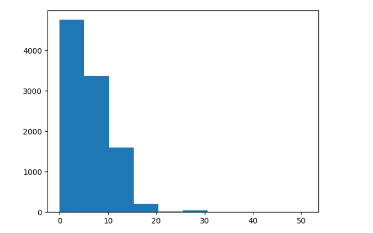
Now find the length of the longest tweet. Remember to look at the training and the validation set.
Exercise 2 - max_len
Calculate the length of the longest tweet.
# GRADED FUNCTION: max_length
def max_length(training_x, validation_x):
    """Computes the length of the longest tweet in the training and validation sets.

    Args:
        training_x (list): The tweets in the training set.
        validation_x (list): The tweets in the validation set.

    Returns:
        int: Length of the longest tweet.
    """
    ### START CODE HERE ###

    max_len = 0

    for tweet in training_x:
        max_len = max(max_len, len(tweet))

    for tweet in validation_x:
        max_len = max(max_len, len(tweet))

    ### END CODE HERE ###
    return max_len

max_len = max_length(train_x, val_x)
print(f'The length of the longest tweet is {max_len} tokens.')
- 1
- 2
- 3
- 4
- 5
- 6
- 7
- 8
- 9
- 10
- 11
- 12
- 13
- 14
- 15
- 16
- 17
- 18
- 19
- 20
- 21
- 22
- 23
- 24
- 25
- 26
Output
The length of the longest tweet is 51 tokens.
- 1
- 2
Expected output:
The length of the longest tweet is 51 tokens.
# Test your max_len function
w1_unittest.test_max_length(max_length)
- 1
- 2
Output
All tests passed
- 1
Exercise 3 - padded_sequence
Implement padded_sequence function to transform sequences of words into padded sequences of numbers. A couple of things to notice:
- The term
tensoris used to refer to the encoded tweet but the function should return a regular python list, not atf.tensor - There is no need to truncate the tweet if it exceeds
max_lenas you already know the maximum length of the tweets beforehand
# GRADED FUNCTION: padded_sequence
def padded_sequence(tweet, vocab_dict, max_len, unk_token='[UNK]'):
    """transform sequences of words into padded sequences of numbers

    Args:
        tweet (list): A single tweet encoded as a list of strings.
        vocab_dict (dict): Vocabulary.
        max_len (int): Length of the longest tweet.
        unk_token (str, optional): Unknown token. Defaults to '[UNK]'.

    Returns:
        list: Padded tweet encoded as a list of int.
    """
    ### START CODE HERE ###

    # Find the ID of the UNK token, to use it when you encounter a new word
    unk_ID = vocab_dict[unk_token]

    # First convert the words to integers by looking up the vocab_dict
    # padded_tensor = []
    #for token in tweet:
    #   padded_tensor.append(vocab_dict[token])
    padded_tensor = [vocab_dict.get(word, unk_ID) for word in tweet]
    # Then pad the tensor with zeroes up to the length max_len
    padded_tensor += [0] * (max_len - len(padded_tensor))

    ### END CODE HERE ###

    return padded_tensor
- 1
- 2
- 3
- 4
- 5
- 6
- 7
- 8
- 9
- 10
- 11
- 12
- 13
- 14
- 15
- 16
- 17
- 18
- 19
- 20
- 21
- 22
- 23
- 24
- 25
- 26
- 27
- 28
- 29
# Test your padded_sequence function
w1_unittest.test_padded_sequence(padded_sequence)
- 1
- 2
Output
All tests passed
- 1
Pad the train and validation dataset
train_x_padded = [padded_sequence(x, vocab, max_len) for x in train_x]
val_x_padded = [padded_sequence(x, vocab, max_len) for x in val_x]
- 1
- 2
3 - Define the structure of the neural network layers
In this part, you will write your own functions and layers for the neural network to test your understanding of the implementation. It will be similar to the one used in Keras and PyTorch. Writing your own small framework will help you understand how they all work and use them effectively in the future.
You will implement the ReLU and sigmoid functions, which you will use as activation functions for the neural network, as well as a fully connected (dense) layer.
3.1 - ReLU
You will now implement the ReLU activation in a function below. The ReLU function looks as follows:
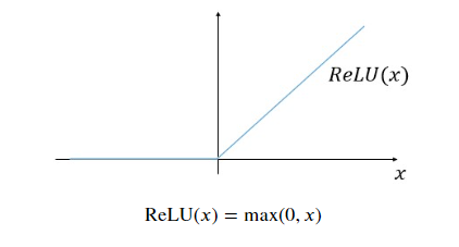
R e L U ( x ) = m a x ( 0 , x ) \mathrm{ReLU}(x) = \mathrm{max}(0,x) ReLU(x)=max(0,x)
Exercise 4 - relu
Instructions: Implement the ReLU activation function below. Your function should take in a matrix or vector and it should transform all the negative numbers into 0 while keeping all the positive numbers intact.
Notice you can get the maximum of two numbers by using np.maximum.
# GRADED FUNCTION: relu
def relu(x):
    '''Relu activation function implementation
    Input:
        - x (numpy array)
    Output:
        - activation (numpy array): input with negative values set to zero
    '''
    ### START CODE HERE ###

    activation = np.maximum(0, x)

    ### END CODE HERE ###

    return activation
- 1
- 2
- 3
- 4
- 5
- 6
- 7
- 8
- 9
- 10
- 11
- 12
- 13
- 14
- 15
# Check the output of your function
x = np.array([[-2.0, -1.0, 0.0], [0.0, 1.0, 2.0]], dtype=float)
print("Test data is:")
print(x)
print("\nOutput of relu is:")
print(relu(x))
- 1
- 2
- 3
- 4
- 5
- 6
Output
Test data is:
[[-2. -1.  0.]
 [ 0.  1.  2.]]

Output of relu is:
[[0. 0. 0.]
 [0. 1. 2.]]
- 1
- 2
- 3
- 4
- 5
- 6
- 7
Expected Output:
Test data is:
[[-2. -1.  0.]
 [ 0.  1.  2.]]

Output of relu is:
[[0. 0. 0.]
 [0. 1. 2.]]
- 1
- 2
- 3
- 4
- 5
- 6
- 7
# Test your relu function
w1_unittest.test_relu(relu)
- 1
- 2
Output
All tests passed
- 1
3.2 - Sigmoid
You will now implement the sigmoid activation in a function below. The sigmoid function looks as follows:
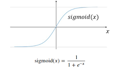
s i g m o i d ( x ) = 1 1 + e − x \mathrm{sigmoid}(x) = \frac{1}{1 + e^{-x}} sigmoid(x)=1+e−x1
Exercise 5 - sigmoid
Instructions: Implement the sigmoid activation function below. Your function should take in a matrix or vector and it should transform all the numbers according to the formula above.
# GRADED FUNCTION: sigmoid
def sigmoid(x):
    '''Sigmoid activation function implementation
    Input:
        - x (numpy array)
    Output:
        - activation (numpy array)
    '''
    ### START CODE HERE ###

    activation = 1 / (1 + np.exp(-x))

    ### END CODE HERE ###

    return activation
- 1
- 2
- 3
- 4
- 5
- 6
- 7
- 8
- 9
- 10
- 11
- 12
- 13
- 14
- 15
# Check the output of your function
x = np.array([[-1000.0, -1.0, 0.0], [0.0, 1.0, 1000.0]], dtype=float)
print("Test data is:")
print(x)
print("\nOutput of sigmoid is:")
print(sigmoid(x))
- 1
- 2
- 3
- 4
- 5
- 6
Output
Test data is:
[[-1000.    -1.     0.]
 [    0.     1.  1000.]]

Output of sigmoid is:
[[0.         0.26894142 0.5       ]
 [0.5        0.73105858 1.        ]]
- 1
- 2
- 3
- 4
- 5
- 6
- 7
Expected Output:
Test data is:
[[-1000.    -1.     0.]
 [    0.     1.  1000.]]

Output of sigmoid is:
[[0.         0.26894142 0.5       ]
 [0.5        0.73105858 1.        ]]
- 1
- 2
- 3
- 4
- 5
- 6
- 7
# Test your sigmoid function
w1_unittest.test_sigmoid(sigmoid)
- 1
- 2
Output: All tests passed
3.3 - Dense Class
Implement the weight initialization in the __init__ method.
- Weights are initialized with a random key.
- The shape of the weights (num_rows, num_cols) should equal the number of columns in the input data (this is in the last column) and the number of units respectively.
- The number of rows in the weight matrix should equal the number of columns in the input data
x. Sincexmay have 2 dimensions if it represents a single training example (row, col), or three dimensions (batch_size, row, col), get the last dimension from the tuple that holds the dimensions of x. - The number of columns in the weight matrix is the number of units chosen for that dense layer.
- The number of rows in the weight matrix should equal the number of columns in the input data
- The values generated should have a mean of 0 and standard deviation of
stdev.- To initialize random weights, a random generator is created using
random_generator = np.random.default_rng(seed=random_seed). This part is implemented for you. You will userandom_generator.normal(...)to create your random weights. Check here how the random generator works. - Please don’t change the
random_seed, so that the results are reproducible for testing (and you can be fairly graded).
- To initialize random weights, a random generator is created using
Implement the forward function of the Dense class.
- The forward function multiplies the input to the layer (
x) by the weight matrix (W)
f o r w a r d ( x , W ) = x W \mathrm{forward}(\mathbf{x},\mathbf{W}) = \mathbf{xW} forward(x,W)=xW
- You can use
numpy.dotto perform the matrix multiplication.
Exercise 6 - Dense
Implement the Dense class. You might want to check how normal random numbers can be generated with numpy by checking the docs.
# GRADED CLASS: Dense
class Dense():
    """
    A dense (fully-connected) layer.
    """

    # Please implement '__init__'
    def __init__(self, n_units, input_shape, activation, stdev=0.1, random_seed=42):

        # Set the number of units in this layer
        self.n_units = n_units
        # Set the random key for initializing weights
        self.random_generator = np.random.default_rng(seed=random_seed)
        self.activation = activation

        ### START CODE HERE ###

        # Generate the weight matrix from a normal distribution and standard deviation of 'stdev'
        # Set the size of the matrix w
        w = self.random_generator.normal(scale=stdev, size = (input_shape[-1], n_units))

        ### END CODE HERE ##

        self.weights = w


    def __call__(self, x):
        return self.forward(x)


    # Please implement 'forward()'
    def forward(self, x):

        ### START CODE HERE ###

        # Matrix multiply x and the weight matrix
        dense = np.dot(x, self.weights)
        # Apply the activation function
        dense = self.activation(dense)

        ### END CODE HERE ###
        return dense
- 1
- 2
- 3
- 4
- 5
- 6
- 7
- 8
- 9
- 10
- 11
- 12
- 13
- 14
- 15
- 16
- 17
- 18
- 19
- 20
- 21
- 22
- 23
- 24
- 25
- 26
- 27
- 28
- 29
- 30
- 31
- 32
- 33
- 34
- 35
- 36
- 37
- 38
- 39
- 40
- 41
- 42
# random_key = np.random.get_prng()  # sets random seed
z = np.array([[2.0, 7.0, 25.0]]) # input array

# Testing your Dense layer
dense_layer = Dense(n_units=10, input_shape=z.shape, activation=relu)  #sets  number of units in dense layer

print("Weights are:\n",dense_layer.weights) #Returns randomly generated weights
print("Foward function output is:", dense_layer(z)) # Returns multiplied values of units and weights
- 1
- 2
- 3
- 4
- 5
- 6
- 7
- 8
Output
Weights are:
 [[ 0.03047171 -0.10399841  0.07504512  0.09405647 -0.19510352 -0.13021795
   0.01278404 -0.03162426 -0.00168012 -0.08530439]
 [ 0.0879398   0.07777919  0.00660307  0.11272412  0.04675093 -0.08592925
   0.03687508 -0.09588826  0.08784503 -0.00499259]
 [-0.01848624 -0.06809295  0.12225413 -0.01545295 -0.04283278 -0.03521336
   0.05323092  0.03654441  0.04127326  0.0430821 ]]
Foward function output is: [[0.21436609 0.         3.25266507 0.59085808 0.         0.
  1.61446659 0.17914382 1.64338651 0.87149558]]
- 1
- 2
- 3
- 4
- 5
- 6
- 7
- 8
- 9
Expected Output:
Weights are:
 [[ 0.03047171 -0.10399841  0.07504512  0.09405647 -0.19510352 -0.13021795
   0.01278404 -0.03162426 -0.00168012 -0.08530439]
 [ 0.0879398   0.07777919  0.00660307  0.11272412  0.04675093 -0.08592925
   0.03687508 -0.09588826  0.08784503 -0.00499259]
 [-0.01848624 -0.06809295  0.12225413 -0.01545295 -0.04283278 -0.03521336
   0.05323092  0.03654441  0.04127326  0.0430821 ]]

Foward function output is: [[0.21436609 0.         3.25266507 0.59085808 0.         0.
  1.61446659 0.17914382 1.64338651 0.87149558]]
- 1
- 2
- 3
- 4
- 5
- 6
- 7
- 8
- 9
- 10
# Test your Dense class
w1_unittest.test_Dense(Dense)
- 1
- 2
Output: All tests passed
3.4 - Model
Now you will implement a classifier using neural networks. Here is the model architecture you will be implementing.
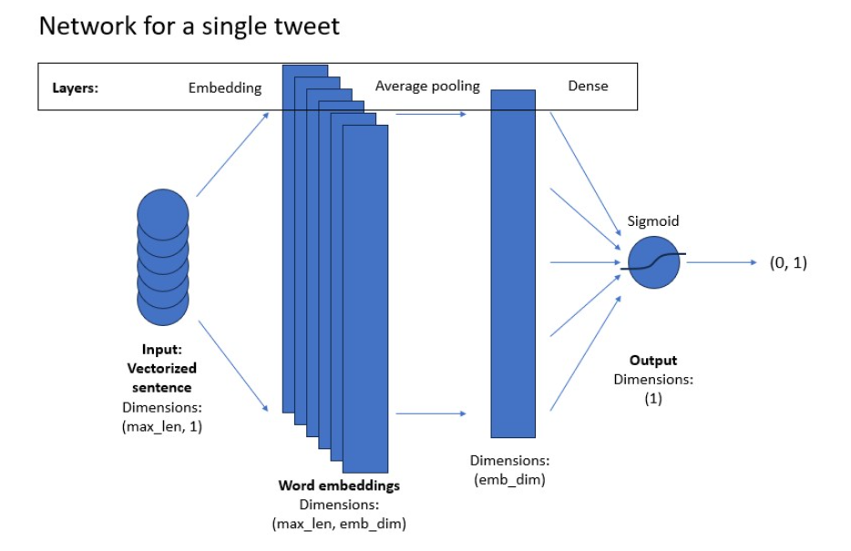
For the model implementation, you will use TensorFlow module, imported as tf. Your model will consist of layers and activation functions that you implemented above, but you will take them directly from the tensorflow library.
You will use the tf.keras.Sequential module, which allows you to stack the layers in a sequence as you want them in the model. You will use the following layers:
- tf.keras.layers.Embedding
- Turns positive integers (word indices) into vectors of fixed size. You can imagine it as creating one-hot vectors out of indices and then running them through a fully-connected (dense) layer.
- tf.keras.layers.GlobalAveragePooling1D
- tf.keras.layers.Dense
- Regular fully connected layer
Please use the help function to view documentation for each layer.
# View documentation on how to implement the layers in tf.
# help(tf.keras.Sequential)
# help(tf.keras.layers.Embedding)
# help(tf.keras.layers.GlobalAveragePooling1D)
# help(tf.keras.layers.Dense)
- 1
- 2
- 3
- 4
- 5
Exercise 7 - create_model
Implement the create_model function.
First you need to create the model. The tf.keras.Sequential has been implemented for you. Within it you should put the following layers:
tf.keras.layers.Embeddingwith the sizenum_wordstimesembeding_dimand theinput_lengthset to the length of the input sequences (which is the length of the longest tweet).tf.keras.layers.GlobalAveragePooling1Dwith no extra parameters.tf.keras.layers.Densewith the size of one (this is your classification output) and'sigmoid'activation passed to theactivationkeyword parameter.
Make sure to separate the layers with a comma.
Then you need to compile the model. Here you can look at all the parameters you can set when compiling the model: tf.keras.Model. In this notebook, you just need to set the loss to 'binary_crossentropy' (because you are doing binary classification with a sigmoid function at the output), the optimizer to 'adam' and the metrics to 'accuracy' (so that you can track the accuracy on the training and validation sets.
# GRADED FUNCTION: create_model
def create_model(num_words, embedding_dim, max_len):
    """
    Creates a text classifier model

    Args:
        num_words (int): size of the vocabulary for the Embedding layer input
        embedding_dim (int): dimensionality of the Embedding layer output
        max_len (int): length of the input sequences

    Returns:
        model (tf.keras Model): the text classifier model
    """

    tf.random.set_seed(123)

    ### START CODE HERE

    model = tf.keras.Sequential([
        tf.keras.layers.Embedding(num_words, embedding_dim, input_length=max_len),
        tf.keras.layers.GlobalAveragePooling1D(),
        tf.keras.layers.Dense(1, activation="sigmoid")
    ])

    model.compile(loss="binary_crossentropy",
                  optimizer="adam",
                  metrics=['accuracy'])

    ### END CODE HERE

    return model
- 1
- 2
- 3
- 4
- 5
- 6
- 7
- 8
- 9
- 10
- 11
- 12
- 13
- 14
- 15
- 16
- 17
- 18
- 19
- 20
- 21
- 22
- 23
- 24
- 25
- 26
- 27
- 28
- 29
- 30
- 31
# Create the model
model = create_model(num_words=num_words, embedding_dim=16, max_len=max_len)

print('The model is created!\n')
- 1
- 2
- 3
- 4
Output: The model is created!
# Test your create_model function
w1_unittest.test_model(create_model)
- 1
- 2
Output: All tests passed
Now you need to prepare the data to put into the model. You already created lists of x and y values and all you need to do now is convert them to NumPy arrays, as this is the format that the model is expecting.
Then you can create a model with the function you defined above and train it. The trained model should give you about 99.6 % accuracy on the validation set.
# Prepare the data
train_x_prepared = np.array(train_x_padded)
val_x_prepared = np.array(val_x_padded)

train_y_prepared = np.array(train_y)
val_y_prepared = np.array(val_y)

print('The data is prepared for training!\n')

# Fit the model
print('Training:')
history = model.fit(train_x_prepared, train_y_prepared, epochs=20, validation_data=(val_x_prepared, val_y_prepared))
- 1
- 2
- 3
- 4
- 5
- 6
- 7
- 8
- 9
- 10
- 11
- 12
Output
The data is prepared for training!

Training:
Epoch 1/20
250/250 [==============================] - 16s 53ms/step - loss: 0.6841 - accuracy: 0.6506 - val_loss: 0.6695 - val_accuracy: 0.9755
Epoch 2/20
250/250 [==============================] - 3s 13ms/step - loss: 0.6358 - accuracy: 0.9386 - val_loss: 0.6008 - val_accuracy: 0.9775
Epoch 3/20
250/250 [==============================] - 1s 4ms/step - loss: 0.5435 - accuracy: 0.9872 - val_loss: 0.5014 - val_accuracy: 0.9900
Epoch 4/20
250/250 [==============================] - 1s 3ms/step - loss: 0.4353 - accuracy: 0.9899 - val_loss: 0.3993 - val_accuracy: 0.9930
Epoch 5/20
250/250 [==============================] - 1s 4ms/step - loss: 0.3370 - accuracy: 0.9941 - val_loss: 0.3119 - val_accuracy: 0.9920
Epoch 6/20
250/250 [==============================] - 1s 3ms/step - loss: 0.2578 - accuracy: 0.9945 - val_loss: 0.2439 - val_accuracy: 0.9955
Epoch 7/20
250/250 [==============================] - 1s 4ms/step - loss: 0.1979 - accuracy: 0.9954 - val_loss: 0.1910 - val_accuracy: 0.9945
Epoch 8/20
250/250 [==============================] - 1s 3ms/step - loss: 0.1533 - accuracy: 0.9961 - val_loss: 0.1518 - val_accuracy: 0.9950
Epoch 9/20
250/250 [==============================] - 1s 3ms/step - loss: 0.1207 - accuracy: 0.9964 - val_loss: 0.1225 - val_accuracy: 0.9950
Epoch 10/20
250/250 [==============================] - 1s 4ms/step - loss: 0.0963 - accuracy: 0.9969 - val_loss: 0.0997 - val_accuracy: 0.9950
Epoch 11/20
250/250 [==============================] - 1s 4ms/step - loss: 0.0780 - accuracy: 0.9969 - val_loss: 0.0826 - val_accuracy: 0.9960
Epoch 12/20
250/250 [==============================] - 1s 2ms/step - loss: 0.0639 - accuracy: 0.9971 - val_loss: 0.0690 - val_accuracy: 0.9965
Epoch 13/20
250/250 [==============================] - 1s 2ms/step - loss: 0.0531 - accuracy: 0.9975 - val_loss: 0.0585 - val_accuracy: 0.9965
Epoch 14/20
250/250 [==============================] - 1s 4ms/step - loss: 0.0446 - accuracy: 0.9976 - val_loss: 0.0500 - val_accuracy: 0.9960
Epoch 15/20
250/250 [==============================] - 1s 4ms/step - loss: 0.0379 - accuracy: 0.9979 - val_loss: 0.0431 - val_accuracy: 0.9960
Epoch 16/20
250/250 [==============================] - 1s 4ms/step - loss: 0.0324 - accuracy: 0.9980 - val_loss: 0.0376 - val_accuracy: 0.9960
Epoch 17/20
250/250 [==============================] - 1s 2ms/step - loss: 0.0280 - accuracy: 0.9980 - val_loss: 0.0327 - val_accuracy: 0.9960
Epoch 18/20
250/250 [==============================] - 1s 3ms/step - loss: 0.0244 - accuracy: 0.9983 - val_loss: 0.0290 - val_accuracy: 0.9960
Epoch 19/20
250/250 [==============================] - 1s 4ms/step - loss: 0.0215 - accuracy: 0.9983 - val_loss: 0.0260 - val_accuracy: 0.9955
Epoch 20/20
250/250 [==============================] - 1s 2ms/step - loss: 0.0189 - accuracy: 0.9983 - val_loss: 0.0233 - val_accuracy: 0.9955
- 1
- 2
- 3
- 4
- 5
- 6
- 7
- 8
- 9
- 10
- 11
- 12
- 13
- 14
- 15
- 16
- 17
- 18
- 19
- 20
- 21
- 22
- 23
- 24
- 25
- 26
- 27
- 28
- 29
- 30
- 31
- 32
- 33
- 34
- 35
- 36
- 37
- 38
- 39
- 40
- 41
- 42
- 43
4 - Evaluate the model
Now that you trained the model, it is time to look at its performance. While training, you already saw a printout of the accuracy and loss on training and validation sets. To have a better feeling on how the model improved with training, you can plot them below.
def plot_metrics(history, metric):
    plt.plot(history.history[metric])
    plt.plot(history.history[f'val_{metric}'])
    plt.xlabel("Epochs")
    plt.ylabel(metric.title())
    plt.legend([metric, f'val_{metric}'])
    plt.show()

plot_metrics(history, "accuracy")
plot_metrics(history, "loss")
- 1
- 2
- 3
- 4
- 5
- 6
- 7
- 8
- 9
- 10
Output
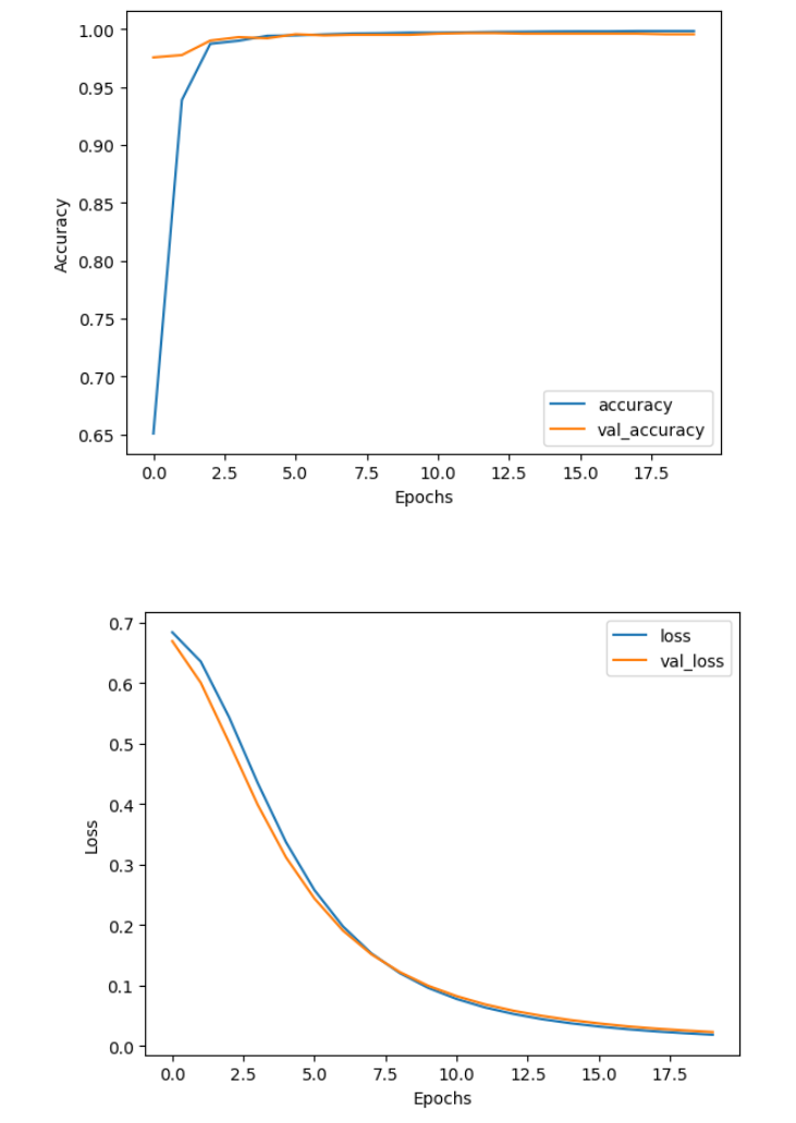
You can see that already after just a few epochs the model reached very high accuracy on both sets. But if you zoom in, you can see that the performance was still slightly improving on the training set through all 20 epochs, while it stagnated a bit earlier on the validation set. The loss on the other hand kept decreasing through all 20 epochs, which means that the model also got more confident in its predictions.
4.1 - Predict on Data
Now you can use the model for predictions on unseen tweets as model.predict(). This is as simple as passing an array of sequences you want to predict to the mentioned method.
In the cell below you prepare an extract of positive and negative samples from the validation set (remember, the positive examples are at the beginning and the negative are at the end) for the demonstration and predict their values with the model. Note that in the ideal case you should have another test set from which you would draw this data to inspect the model performance. But for the demonstration here the validation set will do just as well.
# Prepare an example with 10 positive and 10 negative tweets.
example_for_prediction = np.append(val_x_prepared[0:10], val_x_prepared[-10:], axis=0)

# Make a prediction on the tweets.
model.predict(example_for_prediction)
- 1
- 2
- 3
- 4
- 5
Output
1/1 [==============================] - 0s 67ms/step
- 1
Out[40]:
array([[0.9001521 ],
       [0.99429554],
       [0.99702805],
       [0.9513193 ],
       [0.9976744 ],
       [0.9960562 ],
       [0.9919789 ],
       [0.9800092 ],
       [0.9984914 ],
       [0.9983236 ],
       [0.01062678],
       [0.04205199],
       [0.01288154],
       [0.0168143 ],
       [0.01739226],
       [0.00625729],
       [0.01589022],
       [0.00809518],
       [0.02305534],
       [0.03285299]], dtype=float32)
- 1
- 2
- 3
- 4
- 5
- 6
- 7
- 8
- 9
- 10
- 11
- 12
- 13
- 14
- 15
- 16
- 17
- 18
- 19
- 20
You can see that the first 10 numbers are very close to 1, which means the model correctly predicted positive sentiment and the last 10 numbers are all close to zero, which means the model correctly predicted negative sentiment.
5 - Test With Your Own Input
Finally you will test with your own input. You will see that deepnets are more powerful than the older methods you have used before. Although you go close to 100 % accuracy on the first two assignments, you can see even more improvement here.
5.1 - Create the Prediction Function
def get_prediction_from_tweet(tweet, model, vocab, max_len):
    tweet = process_tweet(tweet)
    tweet = padded_sequence(tweet, vocab, max_len)
    tweet = np.array([tweet])

    prediction = model.predict(tweet, verbose=False)

    return prediction[0][0]
- 1
- 2
- 3
- 4
- 5
- 6
- 7
- 8
Now you can write your own tweet and see how the model predicts it. Try playing around with the words - for example change gr8 for great in the sample tweet and see if the score gets higher or lower.
Also Try writing your own tweet and see if you can find what affects the output most.
unseen_tweet = '@DLAI @NLP_team_dlai OMG!!! what a daaay, wow, wow. This AsSiGnMeNt was gr8.'

prediction_unseen = get_prediction_from_tweet(unseen_tweet, model, vocab, max_len)
print(f"Model prediction on unseen tweet: {prediction_unseen}")
- 1
- 2
- 3
- 4
Output
Model prediction on unseen tweet: 0.7467308640480042
- 1
Exercise 8 - graded_very_positive_tweet
Instructions: For your last exercise in this assignment, you need to write a very positive tweet. To pass this exercise, the tweet needs to score at least 0.99 with the model (which means the model thinks it is very positive).
Hint: try some positive words and/or happy smiley faces 声明:本文内容由网友自发贡献,转载请注明出处:【wpsshop博客】
Copyright © 2003-2013 www.wpsshop.cn 版权所有,并保留所有权利。

