
- 12022起重机司机(限门式起重机)试题及模拟考试_关于门式、桥式起重机,下列说法正确的是()。【多选】 a.起重机路基和轨道的铺设应
- 2【C语言】-- 数据结构 -- 插入排序类(直接插入排序,希尔排序)(超详解+动图+源码)_直接插入排序c语言
- 3数据结构单链表最大值_递归算法,返回单链表l中的最大结点值
- 4Unity Hub添加模块问题_unityhub 如何添加模块
- 5MongoDB数据库的导出导入_mongodump导出整个数据库写到用户名密码
- 6GAN生成对抗网络
- 7MongoDB的数据导入和导出功能_宝塔 mongeb 导入dat
- 8如何使用量化机器人进行自动交易?
- 9机器学习常用算法模型总结_阐述机器学习、深度学习等热点研究方向的代表性模型、算法的特点、底层原理及应用
- 10算法力扣刷题记录 十九【15. 三数之和】
深度学习和神经网络_深度学习之神经网络基础(前馈神经网络)
赞
踩

在之前的机器学习的分享中,我们一起去探索了关于传统机器学习的一些重要的模型,从接下来的分享中,我们开始把目光移到深度学习的领域中,看看现在大热的深度学习是如何在各行各业发挥至关重要的作用的。那今天的分享是关于深度学习的基础----前馈神经网络,内容包括:
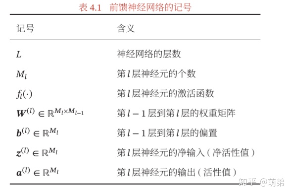
- 神经元
- 激活函数(Activation Function)
- 前馈神经网络
- 反向传播算法
(图片与某些内容来自于邱锡鹏老师的《神经网络与深度学习》与李宏毅老师的深度学习课程)
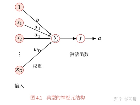
1. 神经元
人工神经元(Artificial Neuron),简称神经元(Neuron),是构成神经网络 的基本单元,其主要是模拟生物神经元的结构和特性,接收一组输入信号并产生输出。
假设一个神经元接受D个输入
净输入z在经过一个非线性函数
其中非线性函数
2. 激活函数(Activation Function)
激活函数 激活函数在神经元中非常重要的。为了增强网络的表示能力和学习能力,激活函数需要具备以下几点性质:
- (1) 连续并可导(允许少数点上不可导)的非线性函数。可导的激活函数可以直接利用数值优化的方法来学习网络参数。
- (2) 激活函数及其导函数要尽可能的简单,有利于提高网络计算效率。
- (3) 激活函数的导函数的值域要在一个合适的区间内,不能太大也不能太小,否则会影响训练的效率和稳定性。
Sigmoid型函数
Sigmoid型函数是指一类S型曲线函数,为两端饱和函数.常用的Sigmoid型函数有Logistic函数和Tanh函数。
Logistic函数
Logistic函数定义为:
Logistic函数可以看成是一个“挤压”函数,把一个实数域的输入“挤压”到 (0, 1).当输入值在0附近时,Sigmoid型函数近似为线性函数;当输入值靠近两端时,对输入进行抑制。输入越小,越接近于0;输入越大,越接近于1。
Tanh函数
Tanh函数也是一种Sigmoid型函数.其定义为
Tanh函数可以看作放大并平移的Logistic函数,其值域是(−1, 1)。
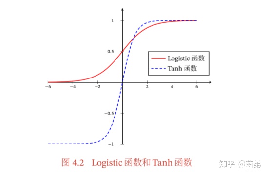
Tanh函数的输出是零中心化的(Zero-Centered),而Logistic函数的输出恒大于0.非零中心化的输出会使得其后一层的神经元的输入发生偏置偏移(Bias Shift),并进一步使得梯度下降的收敛速度变慢。
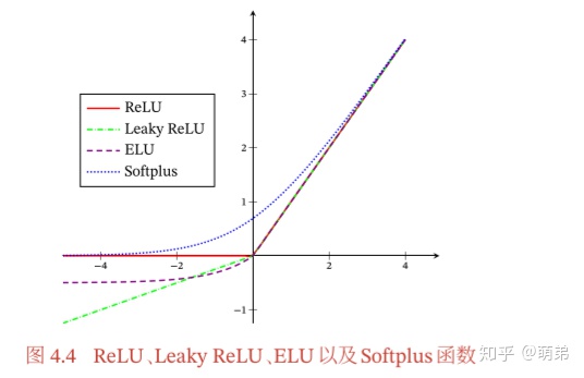
ReLU函数(Rectified Linear Unit,修正线性单元)
ReLU函数
ReLU(Rectified Linear Unit,修正线性单元)是目前深度神经网络中经常使用的激活函数。
ReLU实际上是一个斜坡(ramp)函数,定义为:
- 优点:采用ReLU的神经元只需要进行加、乘和比较的操作,计算上更加高效。Sigmoid型激活函数会导致一个非稀疏的神经网络,而ReLU却具有很好的稀疏性,大约50%的神经元会处于激活状态。
- 缺点:ReLU函数的输出是非零中心化的,给后一层的神经网络引入偏置偏移, 会影响梯度下降的效率。此外,ReLU神经元在训练时比较容易“死亡”.在训练时,如果参数在一次不恰当的更新后,第一个隐藏层中的某个ReLU神经元在所有的训练数据上都不能被激活,那么这个神经元自身参数的梯度永远都会是0,在以后的训练过程中都不会被激活。这种现象较死亡ReLU问题,且有可能发生在其他隐藏层位置。
带泄露的ReLU(Leaky ReLU)
带泄露的ReLU(Leaky ReLU)在输入 < 0时,保持一个很小的梯度
其中
带参数的ReLU(Parametric ReLU,PReLU)
带参数的ReLU(Parametric ReLU,PReLU)引入一个可学习的参数,不 同神经元可以有不同的参数。对于第 个神经元,其PReLU的定义为:
PReLU可以允许不同神经元具有不同的参数,也可以一组神经元共享一个参数。
ELU函数(Exponential Linear Unit,指数线性单元)
ELU(Exponential Linear Unit,指数线性单元)是一个近似的零中心化的非线性函数,其定义为:
其中
Softplus函数
Softplus函数可以看作Rectifier函数的平滑版本,其定义为:
Softplus函数其导数刚好是Logistic函数。Softplus函数虽然也具有单侧抑制、宽兴奋边界的特性,却没有稀疏激活性。
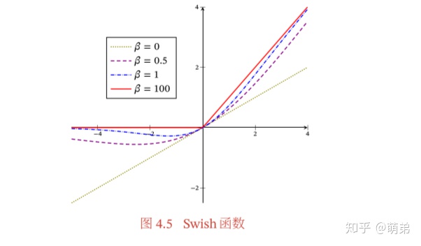
Swish函数
Swish函数是一种自门控(Self-Gated)激活函数,定义为:
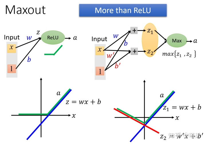
Maxout单元
Maxout单元也是一种分段线性函数。Sigmoid型函数、ReLU等激活函数的输入是神经元的净输入 ,是一个标量.而Maxout单元的输入是上一层神经元的全部原始输出,是一个向量
Maxout单元的过程是:
- 1.输入x与w,得到
- 2.对下一层的神经元分组,如图为两两分组。
- 3.取每个组的最大值作为下一层神经元的输出。
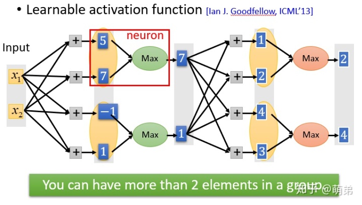
Maxout单元不单是净输入到输出之间的非线性映射,而是整体学习输入到输出之间的非线性映射关系。Maxout激活函数可以看作任意凸函数的分段线性近似,并且在有限的点上是不可微的。
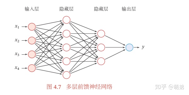
3. 前馈神经网络
前馈网络可以看作一个函数,通过简单非线性函数的多次复合,实现输入空间到输出空间的复杂映射。 在前馈神经网络中,各神经元分别属于不同的层。每一层的神经元可以接收前一层神经元的信号,并产生信号输出到下一层。第0层称为输入层,最后一层称为输出层,其他中间层称为隐藏层.整个网络中无反馈,信号从输入层向输出层单向传播,可用一个有向无环图表示。
这样,前馈神经网络可以通过逐层的信息传递,得到网络最后的输出
其中 , 表示网络中所有层的连接权重和偏置。
通用近似定理
前馈神经网络具有很强的拟合能力,常见的连续非线性函数都可以用前馈神经网络来近似。
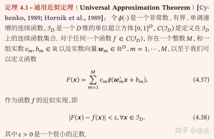
根据通用近似定理,对于具有线性输出层和至少一个使用“挤压”性质的激活函数的隐藏层组成的前馈神经网络,只要其隐藏层神经元的数量足够,它可以以任意的精度来近似任何一个定义在实数空间ℝ 中的有界闭集函数。但是这个定理只给出了任意近似的可行性,但是没有说明近似的效率与是否是最优的,也没有给出找到最优结构的方法,因此我们需要考虑深度的网络而不是用很多个神经元的单个隐藏层的神经网络。
参数学习
给定训练集为
其中 和 分别表示网络中所有的权重矩阵和偏置向量;
Frobenius范数:
有了学习准则和训练样本,网络参数可以通过梯度下降法来进行学习.在梯度下降方法的每次迭代中,第
其中
梯度下降法需要计算损失函数对参数的偏导数,如果通过链式法则逐一对 每个参数进行求偏导比较低效.在神经网络的训练中经常使用反向传播算法来高效地计算梯度。
4. 反向传播算法
假设采用随机梯度下降进行神经网络参数学习,给定一个样本( , ),将 输入到神经网络模型中,得到网络输出为
根据链式法则:
其中,
- 1.计算偏导数
由于
- 2.计算偏导数
由于
为
- 3.计算偏导数
偏导数
误差项
因此:
其中
可以看出,第
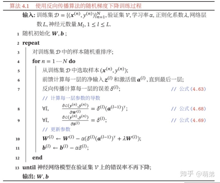
因此, 使用误差反向传播算法的前馈神经网络训练过程可以分为以下三步:
- (1) 前馈计算每一层的净输入 ( ) 和激活值 ( ),直到最后一层;
- (2) 反向传播计算每一层的误差项 ( );
- (3) 计算每一层参数的偏导数,并更新参数。
给出使用反向传播算法的随机梯度下降训练过程:
下面给出部分代码:
- import numpy as np
- import sys
- import os
-
- class NeuralNetMLP(object):
- """ Feedforward neural network / Multi-layer perceptron classifier.
- Parameters
- ------------
- n_hidden : int (default: 30)
- Number of hidden units.
- l2 : float (default: 0.)
- Lambda value for L2-regularization.
- No regularization if l2=0. (default)
- epochs : int (default: 100)
- Number of passes over the training set.
- eta : float (default: 0.001)
- Learning rate.
- shuffle : bool (default: True)
- Shuffles training data every epoch if True to prevent circles.
- minibatch_size : int (default: 1)
- Number of training samples per minibatch.
- seed : int (default: None)
- Random seed for initalizing weights and shuffling.
- Attributes
- -----------
- eval_ : dict
- Dictionary collecting the cost, training accuracy,
- and validation accuracy for each epoch during training.
- """
- def __init__(self, n_hidden=30,
- l2=0., epochs=100, eta=0.001,
- shuffle=True, minibatch_size=1, seed=None):
-
- self.random = np.random.RandomState(seed)
- self.n_hidden = n_hidden
- self.l2 = l2
- self.epochs = epochs
- self.eta = eta
- self.shuffle = shuffle
- self.minibatch_size = minibatch_size
-
- def _onehot(self, y, n_classes):
- """Encode labels into one-hot representation
- Parameters
- ------------
- y : array, shape = [n_samples]
- Target values.
- Returns
- -----------
- onehot : array, shape = (n_samples, n_labels)
- """
- onehot = np.zeros((n_classes, y.shape[0]))
- for idx, val in enumerate(y.astype(int)):
- onehot[val, idx] = 1.
- return onehot.T
-
- def _sigmoid(self, z):
- """Compute logistic function (sigmoid)"""
- return 1. / (1. + np.exp(-np.clip(z, -250, 250)))
-
- def _forward(self, X):
- """Compute forward propagation step"""
-
- # step 1: net input of hidden layer
- # [n_samples, n_features] dot [n_features, n_hidden]
- # -> [n_samples, n_hidden]
- z_h = np.dot(X, self.w_h) + self.b_h
-
- # step 2: activation of hidden layer
- a_h = self._sigmoid(z_h)
-
- # step 3: net input of output layer
- # [n_samples, n_hidden] dot [n_hidden, n_classlabels]
- # -> [n_samples, n_classlabels]
-
- z_out = np.dot(a_h, self.w_out) + self.b_out
-
- # step 4: activation output layer
- a_out = self._sigmoid(z_out)
-
- return z_h, a_h, z_out, a_out
-
- def _compute_cost(self, y_enc, output):
- """Compute cost function.
- Parameters
- ----------
- y_enc : array, shape = (n_samples, n_labels)
- one-hot encoded class labels.
- output : array, shape = [n_samples, n_output_units]
- Activation of the output layer (forward propagation)
- Returns
- ---------
- cost : float
- Regularized cost
- """
- L2_term = (self.l2 *
- (np.sum(self.w_h ** 2.) +
- np.sum(self.w_out ** 2.)))
-
- term1 = -y_enc * (np.log(output))
- term2 = (1. - y_enc) * np.log(1. - output)
- cost = np.sum(term1 - term2) + L2_term
-
- # If you are applying this cost function to other
- # datasets where activation
- # values maybe become more extreme (closer to zero or 1)
- # you may encounter "ZeroDivisionError"s due to numerical
- # instabilities in Python & NumPy for the current implementation.
- # I.e., the code tries to evaluate log(0), which is undefined.
- # To address this issue, you could add a small constant to the
- # activation values that are passed to the log function.
- #
- # For example:
- #
- # term1 = -y_enc * (np.log(output + 1e-5))
- # term2 = (1. - y_enc) * np.log(1. - output + 1e-5)
-
- return cost
-
- def predict(self, X):
- """Predict class labels
- Parameters
- -----------
- X : array, shape = [n_samples, n_features]
- Input layer with original features.
- Returns:
- ----------
- y_pred : array, shape = [n_samples]
- Predicted class labels.
- """
- z_h, a_h, z_out, a_out = self._forward(X)
- y_pred = np.argmax(z_out, axis=1)
- return y_pred
-
- def fit(self, X_train, y_train, X_valid, y_valid):
- """ Learn weights from training data.
- Parameters
- -----------
- X_train : array, shape = [n_samples, n_features]
- Input layer with original features.
- y_train : array, shape = [n_samples]
- Target class labels.
- X_valid : array, shape = [n_samples, n_features]
- Sample features for validation during training
- y_valid : array, shape = [n_samples]
- Sample labels for validation during training
- Returns:
- ----------
- self
- """
- n_output = np.unique(y_train).shape[0] # number of class labels
- n_features = X_train.shape[1]
-
- ########################
- # Weight initialization
- ########################
-
- # weights for input -> hidden
- self.b_h = np.zeros(self.n_hidden)
- self.w_h = self.random.normal(loc=0.0, scale=0.1,
- size=(n_features, self.n_hidden))
-
- # weights for hidden -> output
- self.b_out = np.zeros(n_output)
- self.w_out = self.random.normal(loc=0.0, scale=0.1,
- size=(self.n_hidden, n_output))
-
- epoch_strlen = len(str(self.epochs)) # for progress formatting
- self.eval_ = {'cost': [], 'train_acc': [], 'valid_acc': []}
-
- y_train_enc = self._onehot(y_train, n_output)
-
- # iterate over training epochs
- for i in range(self.epochs):
-
- # iterate over minibatches
- indices = np.arange(X_train.shape[0])
-
- if self.shuffle:
- self.random.shuffle(indices)
-
- for start_idx in range(0, indices.shape[0] - self.minibatch_size +
- 1, self.minibatch_size):
- batch_idx = indices[start_idx:start_idx + self.minibatch_size]
-
- # forward propagation
- z_h, a_h, z_out, a_out = self._forward(X_train[batch_idx])
-
- ##################
- # Backpropagation
- ##################
-
- # [n_samples, n_classlabels]
- sigma_out = a_out - y_train_enc[batch_idx]
-
- # [n_samples, n_hidden]
- sigmoid_derivative_h = a_h * (1. - a_h)
-
- # [n_samples, n_classlabels] dot [n_classlabels, n_hidden]
- # -> [n_samples, n_hidden]
- sigma_h = (np.dot(sigma_out, self.w_out.T) *
- sigmoid_derivative_h)
-
- # [n_features, n_samples] dot [n_samples, n_hidden]
- # -> [n_features, n_hidden]
- grad_w_h = np.dot(X_train[batch_idx].T, sigma_h)
- grad_b_h = np.sum(sigma_h, axis=0)
-
- # [n_hidden, n_samples] dot [n_samples, n_classlabels]
- # -> [n_hidden, n_classlabels]
- grad_w_out = np.dot(a_h.T, sigma_out)
- grad_b_out = np.sum(sigma_out, axis=0)
-
- # Regularization and weight updates
- delta_w_h = (grad_w_h + self.l2*self.w_h)
- delta_b_h = grad_b_h # bias is not regularized
- self.w_h -= self.eta * delta_w_h
- self.b_h -= self.eta * delta_b_h
-
- delta_w_out = (grad_w_out + self.l2*self.w_out)
- delta_b_out = grad_b_out # bias is not regularized
- self.w_out -= self.eta * delta_w_out
- self.b_out -= self.eta * delta_b_out
-
- #############
- # Evaluation
- #############
-
- # Evaluation after each epoch during training
- z_h, a_h, z_out, a_out = self._forward(X_train)
-
- cost = self._compute_cost(y_enc=y_train_enc,
- output=a_out)
-
- y_train_pred = self.predict(X_train)
- y_valid_pred = self.predict(X_valid)
-
- train_acc = ((np.sum(y_train == y_train_pred)).astype(np.float) /
- X_train.shape[0])
- valid_acc = ((np.sum(y_valid == y_valid_pred)).astype(np.float) /
- X_valid.shape[0])
-
- sys.stderr.write('r%0*d/%d | Cost: %.2f '
- '| Train/Valid Acc.: %.2f%%/%.2f%% ' %
- (epoch_strlen, i+1, self.epochs, cost,
- train_acc*100, valid_acc*100))
- sys.stderr.flush()
-
- self.eval_['cost'].append(cost)
- self.eval_['train_acc'].append(train_acc)
- self.eval_['valid_acc'].append(valid_acc)
-
- return self

5. 结语
本期的深度学习基础(前馈神经网络)分享的内容就结束啦,那么从下一期开始,我们就进入卷积神经网络的分享啦,后面会有非常有趣的小案例分享给大家哦,敬请期待。
邱锡鹏:《神经网络与深度学习》
李宏毅:机器学习课程

