[机器学习]简单线性回归——最小二乘法

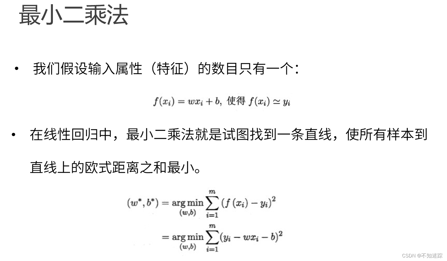
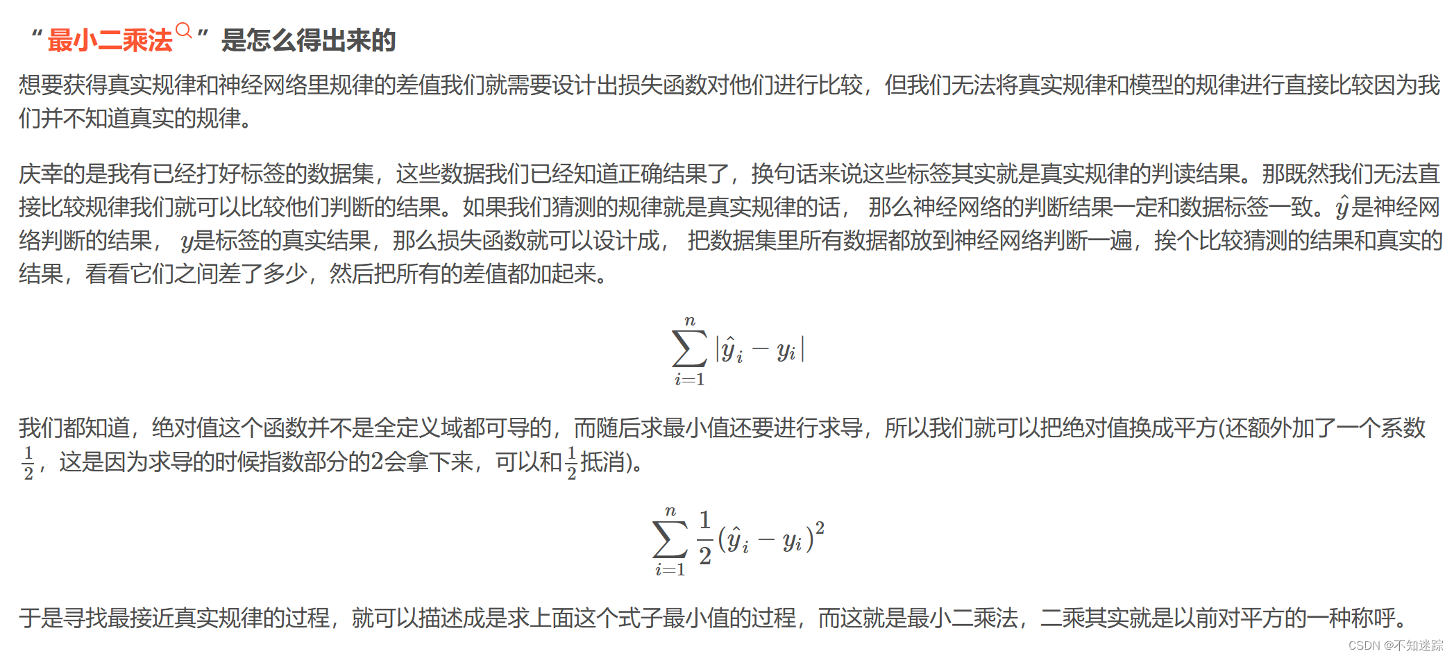
一.线性回归及最小二乘法概念 

2.代码实现 

# 0.引入依赖
import numpy as np
import matplotlib.pyplot as plt
 
# 1.导入数据
points = np.genfromtxt('data.csv', delimiter=',')
# points[0,0]
 
# 提取points中的两列数据，分别作为x，y
x = points[:, 0]
y = points[:, 1]
 
# 用plt画出散点图
# plt.scatter(x, y)
# plt.show()
 
# 2.定义损失函数：最小平方损失函数
# 损失函数是系数的函数，另外还要传入数据的x，y
def compute_cost(w, b, points):
    total_cost = 0
    M = len(points)
 
    # 逐点计算平方损失误差，然后求平均数
    for i in range(M):
        x = points[i, 0]
        y = points[i, 1]
        total_cost += (y - w * x - b) ** 2
 
    return total_cost / M
 
# 3.定义算法拟合函数
# 先定义一个求均值的函数
def average(data):
    sum = 0
    num = len(data)
    for i in range(num):
        sum += data[i]
    return sum / num
 
 
# 定义核心拟合函数
def fit(points):
    M = len(points)
    x_bar = average(points[:, 0])
 
    sum_yx = 0
    sum_x2 = 0
    sum_delta = 0
 
    for i in range(M):
        x = points[i, 0]
        y = points[i, 1]
        sum_yx += y * (x - x_bar)
        sum_x2 += x ** 2
    # 根据公式计算w
    w = sum_yx / (sum_x2 - M * (x_bar ** 2))
 
    for i in range(M):
        x = points[i, 0]
        y = points[i, 1]
        sum_delta += (y - w * x)
    b = sum_delta / M
 
    return w, b
 
# 4.测试
w, b = fit(points)
print("w is: ", w)
print("b is: ", b)
cost = compute_cost(w, b, points)
print("cost is: ", cost)
 
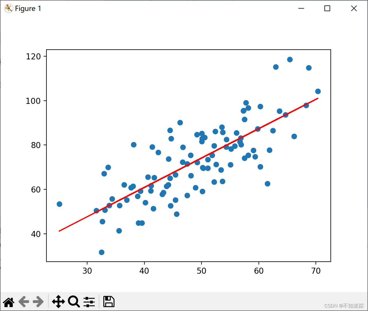
# 5.画出拟合曲线
plt.scatter(x, y)
# 针对每一个x，计算出预测的y值
pred_y = w * x + b
plt.plot(x, pred_y, c='r')
plt.show()

import numpy as np
import matplotlib.pyplot as plt
from sklearn.linear_model import LinearRegression # sklearn库实现
 
# 1. 导入数据（data.csv）
points = np.genfromtxt('data.csv', delimiter=',')
points[0,0]
 
# 提取points中的两列数据，分别作为x，y
x = points[:, 0]
y = points[:, 1]
 
# 用plt画出散点图
# plt.scatter(x, y)
# plt.show()
 
# 2. 定义损失函数：最小平方损失函数
# 损失函数是系数的函数，另外还要传入数据的x，y
def compute_cost(w, b, points):
    total_cost = 0
    M = len(points)
 
    # 逐点计算平方损失误差，然后求平均数
    for i in range(M):
        x = points[i, 0]
        y = points[i, 1]
        total_cost += (y - w * x - b) ** 2
 
    return total_cost / M
 
lr = LinearRegression()
x_new = x.reshape(-1, 1) # 将1行数据变为二维数组
y_new = y.reshape(-1, 1)
lr.fit(x_new, y_new)
 
# 3. 从训练好的模型中提取系数和截距：使用的也是最小二乘法
w = lr.coef_[0][0]
b = lr.intercept_[0]
 
print("w is: ", w)
print("b is: ", b)
 
cost = compute_cost(w, b, points)
 
print("cost is: ", cost)
 
plt.scatter(x, y)
# 针对每一个x，计算出预测的y值
pred_y = w * x + b
 
plt.plot(x, pred_y, c='r')
plt.show()

w is:  1.3224310227553846
b is:  7.991020982269173
cost is:  110.25738346621313

3.代码及数据下载

 简单线性回归-最小二乘法资源-CSDN文库