边缘检测算法总结及其python实现——二阶检测算子_python 边缘检测log算法

二阶检测算子
Laplacian算子，Marr-Hildreth（LOG），高斯差分DoG。
1.Laplacian边缘检测
拉普拉斯算子是n维欧几里德空间中的一个二阶微分算子，定义为梯度（▽f）的散度（▽·f）。拉普拉斯算子也是最简单的各向同性微分算子，具有旋转不变性，即将原图像旋转后进行滤波处理给出的结果与先对图像滤波然后再旋转的结果相同。一个二维图像的拉普拉斯算子定义为：

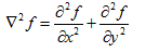
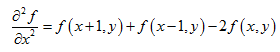
因为任意阶微分都是线性操作，所以拉普拉斯变换也是一个线性算子。为了以离散形式描述这一公式，在x方向将公式描述成：

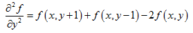
同理，在y方向将公式描述成：

遵循这三个公式，两个变量的离散拉普拉斯算子为：

Laplacian常用的算子模板：
4邻域：

8邻域：

代码：

import numpy as np
from skimage import data,color,filters
import matplotlib.pyplot as plt

original_img=data.chelsea()
gray_img=color.rgb2gray(original_img)

#using system function
edeg_img=filters.laplace(gray_img,ksize=3)

#self codes
w,h = gray_img.shape
ori_pad = np.pad(gray_img,((1,1),(1,1)),'constant')  #在灰度图像的四周填充一行/一列0

lap4_filter = np.array([[0,1,0],[1,-4,1],[0,1,0]])  #4邻域laplacian算子
lap8_filter = np.array([[0,1,0],[1,-8,1],[0,1,0]])  #8邻域laplacian算子

#4邻域
edge4_img = np.zeros((w,h))
for i in range(w-2):
    for j in range(h-2):
        edge4_img[i,j]=np.sum(ori_pad[i:i+3,j:j+3]*lap4_filter)
        if edge4_img[i,j] < 0:
            edge4_img[i,j] = 0  #把所有负值修剪为0

#8邻域
edge8_img = np.zeros((w,h))
for i in range(w-2):
    for j in range(h-2):
        edge8_img[i,j]=np.sum(ori_pad[i:i+3,j:j+3]*lap8_filter)
        if edge8_img[i,j] < 0:
            edge8_img[i,j] = 0

figure=plt.figure()
plt.subplot(231).set_title('original_img')
plt.imshow(original_img)
plt.subplot(232).set_title('gray_image')
plt.imshow(gray_img)
plt.subplot(233).set_title('edge_image')
plt.imshow(edeg_img)
plt.subplot(234).set_title('edge4_image')
plt.imshow(edge4_img)
plt.subplot(235).set_title('edge8_image')
plt.imshow(edge8_img)
plt.show()

1
2
3
4
5
6
7
8
9
10
11
12
13
14
15
16
17
18
19
20
21
22
23
24
25
26
27
28
29
30
31
32
33
34
35
36
37
38
39
40
41
42
43
44
45
46

结果（用封装的函数求出来的结果可能存在一些问题，会继续找问题的所在）：

2.Log边缘检测
拉普拉斯边缘检测算子没有对图像做平滑处理，所以对噪声很敏感。因此可以想到先对图像进行高斯平滑处理，然后再与Laplacian算子进行卷积。这就是高斯拉普拉斯算子(laplacian of gaussian)。

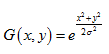
下式中G为标准差为$\sigma$（有时$\sigma$也称为空间常数）的二维高斯函数（省略了常数）

为求${\nabla }^{2}G$的表达式，执行如下微分：
∇ 2 G ( x , y ) = ∂ G ( x , y ) ∂ x 2 + ∂ 2 G ( x , y ) ∂ y 2 = ∂ ∂ x [ − x σ 2 e − x 2 + y 2 2 σ 2 ] + ∂ ∂ y [ − y σ 2 e − x 2 + y 2 2 σ 2 ] = [ x 2 σ 4 − x 2 σ 2 ] e − x 2 + y 2 2 σ 2 + [ y 2 σ 4 − 1 σ 2 ] e − x 2 + y 2 2 σ 2

$$\begin{aligned}\nabla ^{2}G\left( x,y\right) =\dfrac {\partial G\left( x,y\right) }{\partial x^{2}}+\dfrac {\partial ^{2}G\left( x,y\right) }{\partial y^{2}}=\dfrac {\partial }{\partial x} \left[ \dfrac {-x}{\sigma^{2}} e^{-\dfrac {x^{2}+y^{2}}{2\sigma^{2}}}\right] +\dfrac {\partial }{\partial y} \left[ \dfrac{-y}{\sigma^{2}}e^{-\dfrac {x^{2}+y^{2}}{2\sigma^{2}}}\right] \\=\left[ \dfrac {x^{2}}{\sigma^{4}}-\dfrac {x^{2}}{\sigma^{2}}\right]e^{-\dfrac {x^{2}+y^{2}}{2\sigma^{2}}}+\left[ \dfrac {y^{2}}{\sigma^{4}}-\dfrac {1}{\sigma^{2}}\right]e^{-\dfrac {x^{2}+y^{2}}{2\sigma^{2}}}\end{aligned}$$ ∇2G(x,y)=∂x2∂G(x,y)​+∂y2∂2G(x,y)​=∂x∂​⎣⎢⎡​σ2−x​e−2σ2x2+y2​⎦⎥⎤​+∂y∂​⎣⎢⎡​σ2−y​e−2σ2x2+y2​⎦⎥⎤​=[σ4x2​−σ2x2​]e−2σ2x2+y2​+[σ4y2​−σ21​]e−2σ2x2+y2​​
整理各项后给出如下最终表达式：
$${\nabla }^{2}G=\left[-\frac{x^2+y^2-2{\sigma }^2}{{\sigma }^4}\right]e^{-\frac{x^2+y^2}{2{\sigma }^2}}$$
该式成为高斯拉普拉斯（LoG）
Log边缘检测流程：

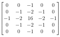
LoG常用的卷积模板是（在实践中，会用该模板的负模板）：

代码：

from skimage import data,color,filters
import matplotlib.pyplot as plt
import numpy as np
original_img=data.chelsea()
gray_img=color.rgb2gray(original_img)

#using system function
g_img=filters.gaussian(gray_img,sigma=0)
system_edge_img=filters.laplace(g_img)
w,h=system_edge_img.shape
for i in range(w):
    for j in range(h):
        if system_edge_img[i][j]<0:
            system_edge_img[i][j]=0

#self codes
g_filter=np.array([[0,0,1,0,0],
                   [0,1,2,1,0],
                   [1,2,16,2,1],
                   [0,1,2,1,0],
                   [0,0,1,0,0]])
self_g_img=np.pad(gray_img,((2,2),(2,2)),'constant')
w,h=self_g_img.shape
for i in range(w-4):
    for j in range(h-4):
        self_g_img[i][j]=np.sum(self_g_img[i:i+5,j:j+5]*g_filter)

lap4_filter = np.array([[0, 1, 0], [1, -4, 1], [0, 1, 0]])  # 4邻域laplacian算子
lap8_filter = np.array([[0, 1, 0], [1, -8, 1], [0, 1, 0]])  # 8邻域laplacian算子

g_pad=np.pad(self_g_img,((1,1),(1,1)),'constant')
# 4邻域
edge4_img = np.zeros((w, h))
for i in range(w - 2):
    for j in range(h - 2):
        edge4_img[i, j] = np.sum(g_pad[i:i + 3, j:j + 3] * lap4_filter)
        if edge4_img[i, j] < 0:
            edge4_img[i, j] = 0  # 把所有负值修剪为0

# 8邻域
edge8_img = np.zeros((w, h))
for i in range(w - 2):
    for j in range(h - 2):
        edge8_img[i, j] = np.sum(g_pad[i:i + 3, j:j + 3] * lap8_filter)
        if edge8_img[i, j] < 0:
            edge8_img[i, j] = 0

figure=plt.figure()
plt.subplot(241).set_title('original_img')
plt.imshow(original_img)
plt.subplot(242).set_title('gray_img')
plt.imshow(gray_img)
plt.subplot(243).set_title('system_g_img')
plt.imshow(g_img)
plt.subplot(244).set_title('self_g_edge')
plt.imshow(self_g_img)
plt.subplot(245).set_title('system_edge')
plt.imshow(system_edge_img)
plt.subplot(246).set_title('edge4_img')
plt.imshow(edge4_img)
plt.subplot(247).set_title('edge8_img')
plt.imshow(edge8_img)
plt.show()
1
2
3
4
5
6
7
8
9
10
11
12
13
14
15
16
17
18
19
20
21
22
23
24
25
26
27
28
29
30
31
32
33
34
35
36
37
38
39
40
41
42
43
44
45
46
47
48
49
50
51
52
53
54
55
56
57
58
59
60
61
62
63

结果：

3.DoG边缘检测
考虑到灰度变化取决于数值范围的事实，有时所用的过程是使用各种$\sigma$值来对一幅图像进行滤波。然后，所得零交叉边缘图与仅为全部图形保留的公共边缘相结合。这种方法可得到很有用的信息，但由于其复杂性，实践中它多被用做使用单一滤波器选择合适的$\sigma$值的设计工具。
Marr and Hildreth[1980]指出过，使用高斯差分（DoG）来近似LoG滤波器是可能的：

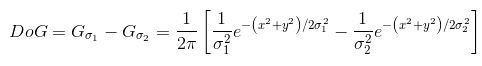
其中$\sigma 1>\sigma 2$。实验结果表明，在人的视觉系统中，某些“通道”就方向和频率而论是有选择性的，且可以使用1.75:1的标准差比率来建模。Marr和Hildreth建议过，使用16:1的比率不仅可保持这些观察的基本特性，而且还可对LoG函数提供一个更接近的“工程”近似。为在LoG和DoG之间进行有意义的比较，对于LoG，$\sigma$值必须按照以下公式选择，以便LoG和DoG具有相同的零交叉：

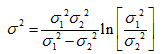
当使用这个$\sigma$值时，尽管LoG和DoG的零交叉相同，但它们的幅度大小会不同。可以通过标定这两个函数使得它们兼容，以便它们在原点处有相同的值。
代码：

from skimage import data,color,filters
import numpy as np
import matplotlib.pyplot as plt
original_img=data.chelsea()
gray_img=color.rgb2gray(original_img)

#先对图像进行两次高斯滤波运算
gimg1=filters.gaussian(gray_img,sigma=2)
gimg2=filters.gaussian(gray_img,sigma=1.6*2)

#两个高斯运算的差分
dimg=gimg2-gimg1

#将差归一化
dimg/=2

figure=plt.figure()
plt.subplot(141).set_title('original_img1')
plt.imshow(original_img)
plt.subplot(142).set_title('LoG_img1')
plt.imshow(gimg1)
plt.subplot(143).set_title('LoG_img2')
plt.imshow(gimg2)
plt.subplot(144).set_title('DoG_edge')
plt.imshow(dimg)
plt.show()
1
2
3
4
5
6
7
8
9
10
11
12
13
14
15
16
17
18
19
20
21
22
23
24
25
26

结果：

各边缘检测算子优缺点比较