花生_TL007

这个屌丝很懒，什么也没留下！

热门标签

【图像分类案例】(1) ResNeXt 交通标志四分类，附Tensorflow完整代码_resnext 模型架构

作者：花生_TL007 | 2024-04-06 17:35:28

踩

resnext 模型架构

各位同学好，今天和大家分享一下如何使用 Tensorflow 构建 ResNeXt 神经网络模型，通过案例实战 ResNeXt 的训练以及预测过程。每个小节的末尾有网络、训练、预测的完整代码。想要数据集的私聊我就行。

ResNeXt 是 ResNet 的改进版，在 bottleneck卷积块结构上进行了较小的改动，其他都和 ResNet 模块相近，如下图所示，ResNeXt 比 ResNet 的精度更好。

本节只介绍 ResNeXt 的改进部分，想了解 ResNet 网络的，可以看我的这篇文章：https://blog.csdn.net/dgvv4/article/details/122396424

1. ResNeXt 模型结构

1.1 分组卷积

（1）在标准卷积中，输入有多少个通道，卷积核就有多少个通道。

举个例子：若输入的图像shape为5x5x6，一个卷积核的shape为3x3x6，使用3个卷积核，得到的特征图shape为3x3x3。参数量 = 5x5x6x3 = 450

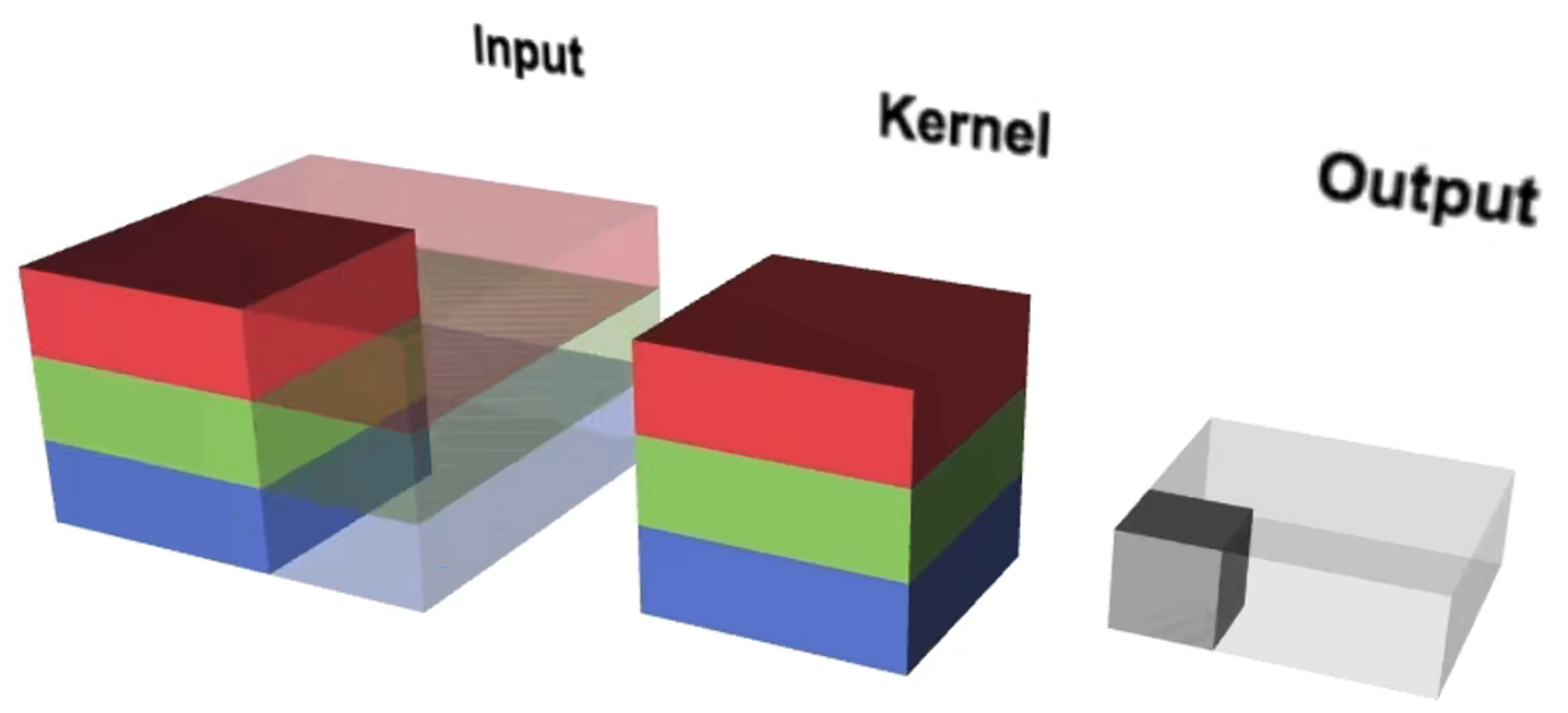
（2）在分组卷积中，每个卷积核只处理部分通道。如下图，红色的卷积核只处理输入图像中红色的两个通道，绿色的卷积核只处理输入图像中间的两个绿色的通道，第三个卷积核只处理黄色的两个通道。此时，每个卷积核有两个通道，每个卷积核生成一个特征图。

举个例子：若输入的图像shape为5x5x6，一个分组卷积核的shape为3x3x2，使用3个分组卷积核，得到的特征图shape为3x3x3。参数量 = 5x5x(6/3)x(3/3)x3 = 5x5x2x1x3 = 150 。可见，分成三组，参数量为原来的三分之一。

因此，分组卷积能够有效地降低参数量和计算量。

代码实现：


#（1）分组卷积块
def group_conv(inputs, filters, stride, num_groups):
    '''
    inputs为输入特征图
    filters为每个分组卷积的输出通道数
    stride为分组卷积的步长
    num_groups为分几组
    '''
    # 用来保存每个分组卷积的输出特征图
    groupList = []
 
    for i in range(num_groups):  # 遍历每一组
        # 均匀取出需要卷积的特征图inputs.shape=[b,h,w,c]
        x = inputs[:, :, :, i*filters: (i+1)*filters]
        # 分别对每一组卷积使用3*3卷积
        x = layers.Conv2D(filters, kernel_size=3, strides=stride, padding='same', use_bias=False)(x)
        # 将每个分组卷积结果保存起来
        groupList.append(x)
    
    # 将每个分组卷积的输出特征图在通道维度上堆叠
    x = layers.Concatenate()(groupList)
 
    x = layers.BatchNormalization()(x)  # 批标准化
 
    x = layers.Activation('relu')(x)  # 激活函数
 
    return x

1.2 残差结构单元

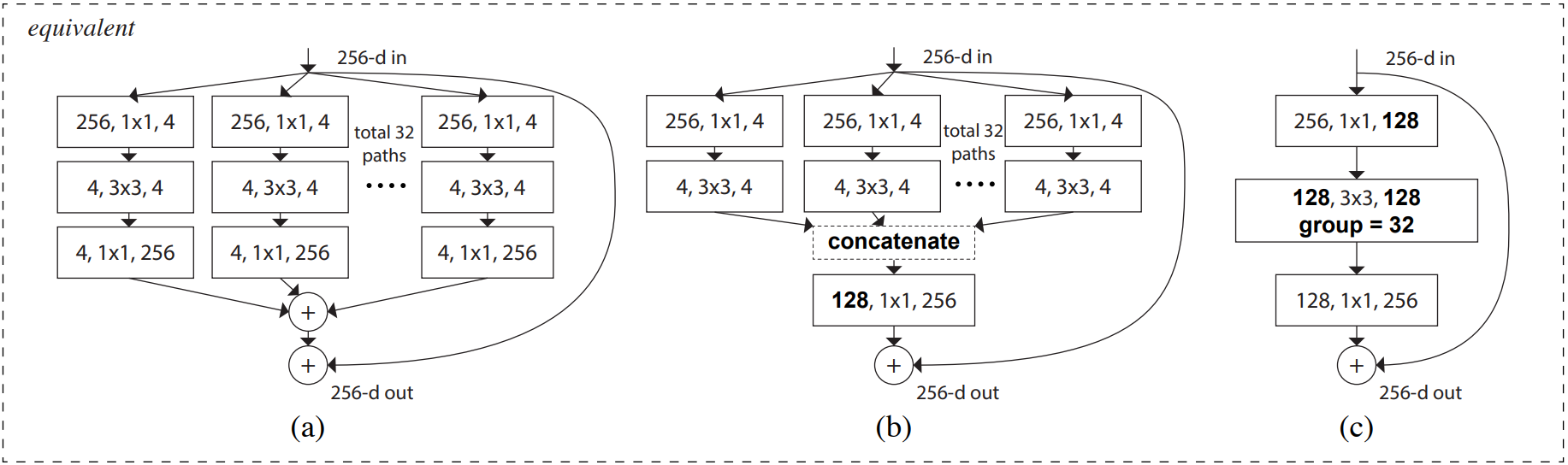
论文中的残差单元结构图如下，它们在数学计算上完全等价。

如图c，首先经过1x1卷积下降通道数 [h,w,256]==>[h,w,128]；然后经过3x3分组卷积提取特征；再经过1x1卷积上升通道数 [h,w,128]==>[h,w,256]；最后，如果输入和输出的shape相同，通过残差连接输入和输出。

如图b，可以理解为，第一层的32个1x1卷积相当于图c的第一个1x1卷积；第二三层的将分组卷积的结果在通道上堆叠，就是图c的3x3分组卷积

代码实现


#（2）一个残差单元
def res_block(inputs, out_channel, stride, shortcut, num_groups=32):
    '''
    inputs输入特征图
    out_channel最后一个1*1卷积的输出通道数
    stride=2下采样, 图像长宽减半, 残差边对输入卷积后再连接输出
    stride=1基本模块, size不变, 残差连接输入和输出
    num_groups代表3*3分组卷积分了几组
    shortcut判断是否要调整通道数
    '''
    # 残差边
    if shortcut is False:  # 直接使用参加连接输入和输出
        residual = inputs
    
    elif shortcut is True:  # 调整通道数
        # 1*1卷积调整通道数，使输入输出的size和通道数相同
        residual = layers.Conv2D(out_channel, kernel_size=1, strides=stride, padding='same', use_bias=False)(inputs)
        # 有BN层就不需要偏置
        residual = layers.BatchNormalization()(residual)
 
    # 1*1卷积，输出通道数是最后一个1*1卷积层输出通道数的一半
    x = layers.Conv2D(filters = out_channel//2, kernel_size=1, strides=1,
                      padding = 'same', use_bias = False)(inputs)
    
    x = layers.BatchNormalization()(x)
    x = layers.Activation('relu')(x)
 
    # 3*3分组卷积
    group_filters = (out_channel//2) // num_groups  # 每一组卷积的输出通道数
    x = group_conv(x, filters = group_filters, stride = stride, num_groups = num_groups)
 
    # 1*1卷积上升通道
    x = layers.Conv2D(filters = out_channel, kernel_size = 1, strides = 1,
                      padding = 'same', use_bias = False)(x)
 
    x = layers.BatchNormalization()(x)
 
    # 残差连接，保证x和残差边的shape相同
    x = layers.Add()([x, residual])
    x = layers.Activation('relu')(x)
 
    return x

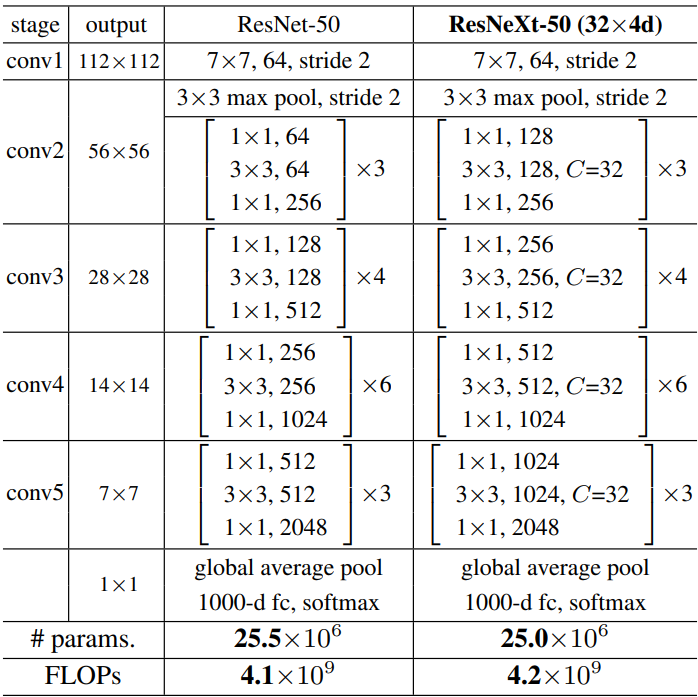
1.3 网络结构

下图是 ResNet 和 ResNeXt 网络结构对比图，接下来就一层一层堆叠网络就可以了

完整代码展示：


import tensorflow as tf
from tensorflow import keras
from tensorflow.keras import layers, Model
 
#（1）分组卷积块
def group_conv(inputs, filters, stride, num_groups):
    '''
    inputs为输入特征图
    filters为每个分组卷积的输出通道数
    stride为分组卷积的步长
    num_groups为分几组
    '''
    # 用来保存每个分组卷积的输出特征图
    groupList = []
 
    for i in range(num_groups):  # 遍历每一组
        # 均匀取出需要卷积的特征图inputs.shape=[b,h,w,c]
        x = inputs[:, :, :, i*filters: (i+1)*filters]
        # 分别对每一组卷积使用3*3卷积
        x = layers.Conv2D(filters, kernel_size=3, strides=stride, padding='same', use_bias=False)(x)
        # 将每个分组卷积结果保存起来
        groupList.append(x)
    
    # 将每个分组卷积的输出特征图在通道维度上堆叠
    x = layers.Concatenate()(groupList)
 
    x = layers.BatchNormalization()(x)  # 批标准化
 
    x = layers.Activation('relu')(x)  # 激活函数
 
    return x
 
#（2）一个残差单元
def res_block(inputs, out_channel, stride, shortcut, num_groups=32):
    '''
    inputs输入特征图
    out_channel最后一个1*1卷积的输出通道数
    stride=2下采样, 图像长宽减半, 残差边对输入卷积后再连接输出
    stride=1基本模块, size不变, 残差连接输入和输出
    num_groups代表3*3分组卷积分了几组
    shortcut判断是否要调整通道数
    '''
    # 残差边
    if shortcut is False:  # 直接使用参加连接输入和输出
        residual = inputs
    
    elif shortcut is True:  # 调整通道数
        # 1*1卷积调整通道数，使输入输出的size和通道数相同
        residual = layers.Conv2D(out_channel, kernel_size=1, strides=stride, padding='same', use_bias=False)(inputs)
        # 有BN层就不需要偏置
        residual = layers.BatchNormalization()(residual)
 
    # 1*1卷积，输出通道数是最后一个1*1卷积层输出通道数的一半
    x = layers.Conv2D(filters = out_channel//2, kernel_size=1, strides=1,
                      padding = 'same', use_bias = False)(inputs)
    
    x = layers.BatchNormalization()(x)
    x = layers.Activation('relu')(x)
 
    # 3*3分组卷积
    group_filters = (out_channel//2) // num_groups  # 每一组卷积的输出通道数
    x = group_conv(x, filters = group_filters, stride = stride, num_groups = num_groups)
 
    # 1*1卷积上升通道
    x = layers.Conv2D(filters = out_channel, kernel_size = 1, strides = 1,
                      padding = 'same', use_bias = False)(x)
 
    x = layers.BatchNormalization()(x)
 
    # 残差连接，保证x和残差边的shape相同
    x = layers.Add()([x, residual])
    x = layers.Activation('relu')(x)
 
    return x
 
#（3）一个残差块
def stage(x, num, out_channel, first_stride):
 
    # 第一个残差单元下采样步长可能是1也可能是2，第一个残差单元需要调整残差边通道数
    x = res_block(x, out_channel, stride=first_stride, shortcut=True)
 
    # 其他的都是基本模块strides=1
    for _ in range(num-1):
        x = res_block(x, out_channel, stride=1, shortcut=False)
 
    # 残差块输出结果
    return x
 
#（4）网络骨架
def resnext(input_shape, classes):
    '''
    input_shape代表输入图像的shape
    classes代表分类类别的数量
    '''
    # 构造输入层
    inputs = keras.Input(shape=input_shape)
 
    # 7*7标准卷积[224,224,3]==>[112,112,64]
    x = layers.Conv2D(filters=64, kernel_size=7, strides=2,
                      padding='same', use_bias=False)(inputs)
    
    x = layers.BatchNormalization()(x)
    x = layers.Activation('relu')(x)
 
    # 最大池化[112,112,64]==>[56,56,64]
    x = layers.MaxPooling2D(pool_size=(3,3), strides=2, padding='same')(x)
 
    # [56,56,64]==>[56,56,256]
    x = stage(x, num=3, out_channel=256, first_stride=1)
 
    # [56,56,256]==>[28,28,512]
    x = stage(x, num=4, out_channel=512, first_stride=2)
 
    # [28,28,512]==>[14,14,1024]
    x = stage(x, num=6, out_channel=1024, first_stride=2)
 
    # [14,14,1024]==>[7,7,2048]
    x = stage(x, num=3, out_channel=2048, first_stride=2)
 
    # [7,7,2048]==>[None,2048]
    x = layers.GlobalAveragePooling2D()(x)
 
    # [None,2048]==>[None,classes]
    logits = layers.Dense(classes)(x)  # 输出不经过softmax激活函数
 
    # 构建模型
    model = Model(inputs, logits)
 
    # 返回模型
    return model
 
#（5）接收网络模型
if __name__ == '__main__':
 
    model = resnext(input_shape = [224,224,3],  # 输入图像shape
                    classes = 1000)  # 分类数
    
    model.summary()  # 查看网络架构

通过model.summary()查看网络参数量


==================================================================================================
Total params: 25,097,128
Trainable params: 25,028,904
Non-trainable params: 68,224
__________________________________________________________________________________________________

2. 模型训练

我是用的GPU训练网络，先将各种包导入进来，并设置GPU内存占用，防止内存爆炸。


from tensorflow.keras.preprocessing.image import ImageDataGenerator  # 预处理
import matplotlib.pyplot as plt
import tensorflow as tf
from tensorflow import keras
from ResNeXt import resnext  # 网络模型
import json
import os
 
os.environ['CUDA_DEVICE_ORDER'] = 'PCI_BUS_ID'  # 调用GPU训练
os.environ['CUDA_VISIBLE_DEVICES'] = '0'  # 使用当前设备的第一块GPU
 
gpus = tf.config.experimental.list_physical_devices("GPU")
 
# 设置GPU内存占用，根据网络模型大小占用相应的内存
if gpus:
    try:
        for gpu in gpus:
            tf.config.experimental.set_memory_growth(gpu, True)
    except RuntimeError as e:
        print(e)
        exit(-1)

2.1 数据集加载

接下来，在文件夹中图片数据以测试集、验证集、测试集分类。

函数 tf.keras.preprocessing.image_dataset_from_directory() 构造数据集，

分批次读取图片数据，参数 img_size 会对读进来的图片resize成指定大小；参数 label_mode 中，'int'代表目标值y是数值类型索引，即0, 1, 2, 3等；'categorical'代表onehot类型，对应正确类别的索引的值为1，如图像属于第二类则表示为0,1,0,0,0；'binary'代表二分类。


#（1）加载数据集
def get_data(height, width, batchsz):
    
    # 训练集数据
    train_ds = keras.preprocessing.image_dataset_from_directory(
        directory = filepath + 'train',  # 训练集图片所在文件夹
        label_mode = 'categorical',  # onehot编码
        image_size = (height, width),  # 输入图象的size
        batch_size = batchsz)  # 每批次训练32张图片
 
    # 验证集数据
    val_ds = keras.preprocessing.image_dataset_from_directory(
        directory = filepath + 'val', 
        label_mode = 'categorical', 
        image_size = (height, width),  
        batch_size = batchsz)  
 
 
    # 返回划分好的数据集
    return train_ds, val_ds
 
# 读取数据集
train_ds, val_ds = get_data(height, width, batchsz)

2.2 显示图像信息

接下来绘图查看图像信息，iter()生成迭代器，配合next()每次运行取出训练集中的一个batch数据。


def plot_show(train_ds):
 
    # 生成迭代器,每次取出一个batch的数据
    sample = next(iter(train_ds))  # sample[0]图像信息, sample[1]标签信息
    # 显示前5张图
    for i in range(5):
        plt.subplot(1,5,i+1)  # 在一块画板的子画板上绘制1行5列
        plt.imshow(sample[0][i]/255.0)  # 图像的像素值压缩到0-1
        plt.xticks([])  # 不显示xy坐标刻度
        plt.yticks([])
    plt.show()
 
# 是否展示图像信息
if plotShow is True:
    plot_show(train_ds)

显示图像如下：

2.3 数据预处理

使用.map()函数转换数据集中所有x和y的类型，并将每张图象的像素值映射到[0,1]之间，打乱训练集数据的顺序.shuffle()


def processing(x,y):  # 定义预处理函数
    x = tf.cast(x, dtype=tf.float32) / 255.0  # 图片转换为tensor类型，并归一化
    y = tf.cast(y, dtype=tf.int32)  # 分类标签转换成tensor类型
    return x,y
 
# 对所有数据预处理
train_ds = train_ds.map(processing).shuffle(10000)  # map调用自定义预处理函数, shuffle打乱数据集
val_ds = val_ds.map(processing)

2.4 网络训练

在网络编译.compile()，指定损失loss采用交叉熵损失。设置参数from_logits=True，由于网络的输出层没有使用softmax函数将输出的实数转为概率，参数设置为True时，会自动将logits的实数转为概率值，再和真实值计算损失，这里的真实值y是经过onehot编码之后的结果。


#（7）保存权重文件
if not os.path.exists(weights_dir):  # 判断当前文件夹下有没有一个叫save_weights的文件夹
    os.makedirs(weights_dir)  # 如果没有就创建一个
 
#（8）模型编译
opt = optimizers.Adam(learning_rate=learning_rate)  # 设置Adam优化器
 
model.compile(optimizer=opt, #学习率
              loss=keras.losses.CategoricalCrossentropy(from_logits=True), # 交叉熵损失，logits层先经过softmax
              metrics=['accuracy']) #评价指标
 
#（9）定义回调函数，一个列表
# 保存模型参数
callbacks = [keras.callbacks.ModelCheckpoint(filepath = 'save_weights/resnext.h5',  # 参数保存的位置
                                            save_best_only = True,  # 保存最佳参数
                                            save_weights_only = True,  # 只保存权重文件
                                            monitor = 'val_loss')]  # 通过验证集损失判断是否是最佳参数
 
#（10）模型训练，history保存训练信息
history = model.fit(x = train_ds,  # 训练集
                    validation_data = val_ds,  # 验证集
                    epochs = epochs,  #迭代30次
                    callbacks = callbacks)

训练过程中的损失值和准确率如下：


Epoch 1/10
556/556 [==============================] - 247s 370ms/step - loss: 1.3545 - accuracy: 0.5662 - val_loss: 0.1252 - val_accuracy: 0.9664
Epoch 2/10
556/556 [==============================] - 175s 305ms/step - loss: 0.1186 - accuracy: 0.9622 - val_loss: 0.1337 - val_accuracy: 0.9724
Epoch 3/10
556/556 [==============================] - 176s 307ms/step - loss: 0.0499 - accuracy: 0.9859 - val_loss: 3.8282 - val_accuracy: 0.6735
Epoch 4/10
556/556 [==============================] - 176s 305ms/step - loss: 0.0697 - accuracy: 0.9816 - val_loss: 0.0783 - val_accuracy: 0.9796
Epoch 5/10
556/556 [==============================] - 176s 306ms/step - loss: 0.1167 - accuracy: 0.9661 - val_loss: 0.0843 - val_accuracy: 0.9844
Epoch 6/10
556/556 [==============================] - 177s 308ms/step - loss: 0.0703 - accuracy: 0.9841 - val_loss: 0.0096 - val_accuracy: 0.9964
Epoch 7/10
556/556 [==============================] - 176s 306ms/step - loss: 0.0267 - accuracy: 0.9920 - val_loss: 0.0295 - val_accuracy: 0.9940
Epoch 8/10
556/556 [==============================] - 176s 306ms/step - loss: 0.0339 - accuracy: 0.9925 - val_loss: 0.0870 - val_accuracy: 0.9712
Epoch 9/10
556/556 [==============================] - 174s 302ms/step - loss: 0.0622 - accuracy: 0.9851 - val_loss: 0.0588 - val_accuracy: 0.9904
Epoch 10/10
556/556 [==============================] - 176s 306ms/step - loss: 0.0384 - accuracy: 0.9889 - val_loss: 3.3135 - val_accuracy: 0.6591

2.5 绘制训练曲线

history 中保存了本轮训练的信息，由于没有使用预训练权重，模型的训练损失和准确率波动比较大，但准确率还是可以的。并且训练时设置了回调函数callbacks，只保存验证集损失最小时的权重参数。


#（11）获取训练信息
history_dict = history.history  # 获取训练的数据字典
train_loss = history_dict['loss']  # 训练集损失
train_accuracy = history_dict['accuracy']  # 训练集准确率
val_loss = history_dict['val_loss']  # 验证集损失
val_accuracy = history_dict['val_accuracy']  # 验证集准确率
 
#（12）绘制训练损失和验证损失
plt.figure()
plt.plot(range(epochs), train_loss, label='train_loss')  # 训练集损失
plt.plot(range(epochs), val_loss, label='val_loss')  # 验证集损失
plt.legend()  # 显示标签
plt.xlabel('epochs')
plt.ylabel('loss')
 
#（13）绘制训练集和验证集准确率
plt.figure()
plt.plot(range(epochs), train_accuracy, label='train_accuracy')  # 训练集准确率
plt.plot(range(epochs), val_accuracy, label='val_accuracy')  # 验证集准确率
plt.legend()
plt.xlabel('epochs')
plt.ylabel('accuracy')

绘制损失曲线和准确率曲线

2.6 训练过程完整代码

训练阶段一定要注意 batch_size 的大小，batch_size 设置的越大，越容易导致显存爆炸，要改的话最好设置2的n次方


import tensorflow as tf
from tensorflow import keras
from tensorflow.keras import optimizers
from ResNeXt import resnext  # 导入模型
import os
import matplotlib.pyplot as plt
 
os.environ['CUDA_DEVICE_ORDER'] = 'PCI_BUS_ID'  # 调用GPU训练
os.environ['CUDA_VISIBLE_DEVICES'] = '0'  # 使用当前设备的第一块GPU
 
gpus = tf.config.experimental.list_physical_devices("GPU")
 
# 设置GPU内存占用，根据网络模型大小占用相应的内存
if gpus:
    try:
        for gpu in gpus:
            tf.config.experimental.set_memory_growth(gpu, True)
    except RuntimeError as e:
        print(e)
        exit(-1)
 
# ------------------------------------- #
# 加载数据集，batchsz太大会导致显存爆炸
# ------------------------------------- #
filepath = 'D:/deeplearning/test/数据集/交通标志/new_data/'  # 数据集所在文件夹
height = 224  # 输入图象的高
width = 224  # 输入图象的宽
batchsz = 8  # 每个batch处理32张图片
checkData = False  # 查看数据集划分的信息
plotShow = True  # 绘制图像
checkDataAgain = False  # 预处理之后是否再次查看数据集信息
# ------------------------------------- #
# 网络模型结构
# ------------------------------------- #
input_shape = (224,224,3)  # 输入图象的shape
classes = 4  # 图像分类的类别数
checkNet = False  # 是否查看网络架构
# ------------------------------------- #
# 网络训练
# ------------------------------------- #
weights_dir = 'save_weights'  # 权重文件保存的文件夹路径
learning_rate = 0.0005  # adam优化器的学习率
epochs = 10  # 训练迭代次数
 
 
#（1）加载数据集
def get_data(height, width, batchsz):
    
    # 训练集数据
    train_ds = keras.preprocessing.image_dataset_from_directory(
        directory = filepath + 'train',  # 训练集图片所在文件夹
        label_mode = 'categorical',  # onehot编码
        image_size = (height, width),  # 输入图象的size
        batch_size = batchsz)  # 每批次训练32张图片
 
    # 验证集数据
    val_ds = keras.preprocessing.image_dataset_from_directory(
        directory = filepath + 'val', 
        label_mode = 'categorical', 
        image_size = (height, width),  
        batch_size = batchsz)  
 
 
    # 返回划分好的数据集
    return train_ds, val_ds
 
# 读取数据集
train_ds, val_ds = get_data(height, width, batchsz) 
 
#（2）查看数据集信息
def check_data(train_ds):  # 传入训练集数据集
    
    # 查看数据集有几个分类类别
    class_names = train_ds.class_names
    print('classNames:', class_names)
 
    # 查看数据集的shape, x代表图片数据, y代表分类类别数据
    sample = next(iter(train_ds))  # 生成迭代器,每次取出一个batch的数据
    print('x_batch.shape:', sample[0].shape, 'y_batch.shape:', sample[1].shape)
    print('前五个目标值:', sample[1][:5])
 
# 是否查看数据集信息
if checkData is True:
    check_data(train_ds)
 
 
#（3）查看图像
def plot_show(train_ds):
 
    # 生成迭代器,每次取出一个batch的数据
    sample = next(iter(train_ds))  # sample[0]图像信息, sample[1]标签信息
    # 显示前5张图
    for i in range(5):
        plt.subplot(1,5,i+1)  # 在一块画板的子画板上绘制1行5列
        plt.imshow(sample[0][i])  # 图像的像素值压缩到0-1
        plt.xticks([])  # 不显示xy坐标刻度
        plt.yticks([])
    plt.show()
 
# 是否展示图像信息
if plotShow is True:
    plot_show(train_ds)
 
 
#（4）数据预处理
def processing(x,y):  # 定义预处理函数
    x = tf.cast(x, dtype=tf.float32) / 255.0  # 图片转换为tensor类型，并归一化
    y = tf.cast(y, dtype=tf.int32)  # 分类标签转换成tensor类型
    return x,y
 
# 对所有数据预处理
train_ds = train_ds.map(processing).shuffle(10000)  # map调用自定义预处理函数, shuffle打乱数据集
val_ds = val_ds.map(processing)
 
 
#（5）查看预处理后的数据是否正确
def check_data_again(train_ds):  # 传入训练集数据集
 
    sample = next(iter(train_ds))  # 生成迭代器,每次取出一个batch的数据
    print('-------after preprocessing-------')
    print('x_batch.shape:', sample[0].shape, 'y_batch.shape:', sample[1].shape)
    print('前五个目标值:', sample[1][:5])
 
# 是否查看数据集信息
if checkDataAgain is True:
    check_data_again(train_ds)
 
 
#（6）导入网络模型
model = resnext(input_shape=input_shape, # 网络的输入图像的size
                classes=classes)  # 分类数
 
# 查看网络构架
if checkNet is True:
    model.summary()
 
 
#（7）保存权重文件
if not os.path.exists(weights_dir):  # 判断当前文件夹下有没有一个叫save_weights的文件夹
    os.makedirs(weights_dir)  # 如果没有就创建一个
 
 
#（8）模型编译
opt = optimizers.Adam(learning_rate=learning_rate)  # 设置Adam优化器
 
model.compile(optimizer=opt, #学习率
              loss=keras.losses.CategoricalCrossentropy(from_logits=True), # 交叉熵损失，logits层先经过softmax
              metrics=['accuracy']) #评价指标
 
 
#（9）定义回调函数，一个列表
# 保存模型参数
callbacks = [keras.callbacks.ModelCheckpoint(filepath = 'save_weights/resnext.h5',  # 参数保存的位置
                                            save_best_only = True,  # 保存最佳参数
                                            save_weights_only = True,  # 只保存权重文件
                                            monitor = 'val_loss')]  # 通过验证集损失判断是否是最佳参数
 
 
#（10）模型训练，history保存训练信息
history = model.fit(x = train_ds,  # 训练集
                    validation_data = val_ds,  # 验证集
                    epochs = epochs,  #迭代30次
                    callbacks = callbacks) 
 
 
#（11）获取训练信息
history_dict = history.history  # 获取训练的数据字典
train_loss = history_dict['loss']  # 训练集损失
train_accuracy = history_dict['accuracy']  # 训练集准确率
val_loss = history_dict['val_loss']  # 验证集损失
val_accuracy = history_dict['val_accuracy']  # 验证集准确率
 
#（12）绘制训练损失和验证损失
plt.figure()
plt.plot(range(epochs), train_loss, label='train_loss')  # 训练集损失
plt.plot(range(epochs), val_loss, label='val_loss')  # 验证集损失
plt.legend()  # 显示标签
plt.xlabel('epochs')
plt.ylabel('loss')
 
#（13）绘制训练集和验证集准确率
plt.figure()
plt.plot(range(epochs), train_accuracy, label='train_accuracy')  # 训练集准确率
plt.plot(range(epochs), val_accuracy, label='val_accuracy')  # 验证集准确率
plt.legend()
plt.xlabel('epochs')
plt.ylabel('accuracy')

3. 预测阶段

以对整个测试集的图片预测为例，test_ds 存放测试集的图片和类别标签，对测试集进行和训练集相同的预处理方法，将像素值映射到0-1之间。

model.predict(img) 返回的是每张图片属于每个类别的概率，需要找到概率最大值所对应的索引 np.argmax(result)，该索引对应的分类名称就是最终预测结果。

打印前10组预测结果


真实值:  ['forbiden', 'forbiden', 'slow', 'forbiden', 'goahead', 'slow', 'goahead', 'slow', 'slow', 'forbiden']
预测值:  ['forbiden', 'forbiden', 'slow', 'forbiden', 'goahead', 'slow', 'goahead', 'slow', 'slow', 'forbiden']

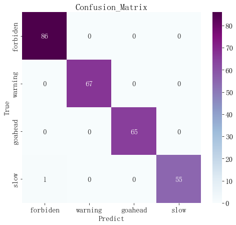
生成真实值和预测值的对比热力图可以观察整个测试集的预测情况

完整代码如下：


import tensorflow as tf
from tensorflow import keras
from ResNeXt import resnext
from PIL import Image
import numpy as np
import matplotlib.pyplot as plt
 
# 报错解决：NotFoundError: No algorithm worked! when using Conv2D
from tensorflow.compat.v1 import ConfigProto
from tensorflow.compat.v1 import InteractiveSession
config = ConfigProto()
config.gpu_options.allow_growth = True
session = InteractiveSession(config=config)
 
 
# ------------------------------------ #
# 预测参数设置
# ------------------------------------ #
im_height = 224  # 输入图像的高
im_width = 224   # 输入图像的高
# 分类名称
class_names = ['forbiden', 'warning', 'goahead', 'slow']
# 权重路径
weight_dir = 'save_weights/resnext.h5'
 
# ------------------------------------ #
# 单张图片预测
# ------------------------------------ #
# 是否只预测一张图
single_pic = False
# 图像所在文件夹的路径
single_filepath = 'D:/deeplearning/test/数据集/交通标志/new_data/test/禁令标志/'  
# 指定某张图片
picture = single_filepath + '010_0001.png'
 
# ------------------------------------ #
# 对测试集图片预测
# ------------------------------------ #
test_pack = True
# 验证集文件夹路径
test_filepath = 'D:/deeplearning/test/数据集/交通标志/new_data/test/'
 
 
#（1）载入模型
model = resnext(input_shape=[224,224,3], classes=4)  # 模型的输入shape和输出分类数
print('model is loaded')
 
#（2）载入权重.h文件
model.load_weights(weight_dir)
print('weights is loaded')
 
#（3）只对单张图像预测
if single_pic is True:
    
    # 加载图片
    img = Image.open(picture)
    # 改变图片size
    img = img.resize((im_height, im_width))
    # 展示图像
    plt.figure()
    plt.imshow(img)
    plt.xticks([])
    plt.yticks([])
    
    # 图像像素值归一化处理
    img = np.array(img) / 255.0
    
    # 输入网络的要求，给图像增加一个batch维度, [h,w,c]==>[b,h,w,c]
    img = np.expand_dims(img, axis=0)
 
    # 预测图片，返回结果包含batch维度[b,n]
    result = model.predict(img)
    # 转换成一维，挤压掉batch维度
    result = np.squeeze(result)
    
    # 找到概率最大值对应的索引
    predict_class = np.argmax(result)
    
    # 打印预测类别及概率
    print('class:', class_names[predict_class], 
          'prob:', result[predict_class])
    
    plt.title(f'{class_names[predict_class]}')
    plt.show()
 
#（4）对测试集图像预测
if test_pack is True:
    
    # 载入测试集
    test_ds = keras.preprocessing.image_dataset_from_directory(
        directory = test_filepath, 
        label_mode = 'int',  # 不经过ont编码, 1、2、3、4、、、 
        image_size = (im_height, im_width),  # 测试集的图像resize
        batch_size = 32)  # 每批次32张图
    
    # 测试机预处理
    #（2）数据预处理
    def processing(image, label): 
        image = tf.cast(image, tf.float32) / 255.0  #[0,1]之间
        label = tf.cast(label, tf.int32)  # 修改数据类型
        return (image, label)
 
    test_ds = test_ds.map(processing) # 预处理
 
 
    test_true = []  # 存放真实值
    test_pred = []  # 存放预测值
    
    # 遍历测试集所有的batch
    for imgs, labels in test_ds:
        # 每次每次取出一个batch的一张图像和一个标签
        for img, label in zip(imgs, labels):
            
            # 网络输入的要求，给图像增加一个维度[h,w,c]==>[b,h,w,c]
            image_array = tf.expand_dims(img, axis=0)
            # 预测某一张图片，返回图片属于许多类别的概率
            prediction = model.predict(image_array)
            
            # 找到预测概率最大的索引对应的类别
            test_pred.append(class_names[np.argmax(prediction)])
            # label是真实标签索引
            test_true.append(class_names[label])
            
    # 展示结果
    print('真实值: ', test_true[:10])
    print('预测值: ', test_pred[:10])
    
    # 绘制混淆矩阵
    from sklearn.metrics import confusion_matrix
    import seaborn as sns
    import pandas as pd
    plt.rcParams['font.sans-serif'] = ['SimSun']  #宋体
    plt.rcParams['font.size'] = 15  #设置字体大小
    
    # 生成混淆矩阵
    conf_numpy = confusion_matrix(test_true, test_pred)
    # 转换成DataFrame表格类型，设置行列标签
    conf_df = pd.DataFrame(conf_numpy, index=class_names, columns=class_names)
    
    # 创建绘图区
    plt.figure(figsize=(8,7))
    
    # 生成热力图
    sns.heatmap(conf_df, annot=True, fmt="d", cmap="BuPu")
    
    # 设置标签
    plt.title('Confusion_Matrix')
    plt.xlabel('Predict')
    plt.ylabel('True')

声明：本文内容由网友自发贡献，不代表【wpsshop博客】立场，版权归原作者所有，本站不承担相应法律责任。如您发现有侵权的内容，请联系我们。转载请注明出处：https://www.wpsshop.cn/w/花生_TL007/article/detail/373334