MATLAB机器人工具箱使用

MATLAB机器人工具箱（一）

前言：

    在开始做机器人仿真之前，我了解了一系列机器人仿真软件（包括Matlab、Webots、Gazebo、V-rep、Adams、Simbad、Morse等）的适用场景、使用方法等资料，决定从最经典的Matlab入手，快速搭建机器人平台进行路径规划与控制。
    这里记录一下我的学习和使用过程，以及遇到的坑。我的版本是R2018a。

---

一、添加机器人工具箱——RTB工具箱：

方法一：
    1.下载rvctools文件包，放在一个自己知道的目录下(任意路径都是可以的，但是为了方便管理，一般都安装在toolbox)，然后“设置路径”里面添加并保存。

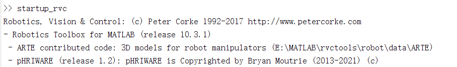
    2.在命令中输入statrup_rvc，之后会看到机器人工具箱启动成功。

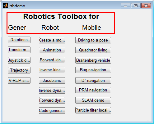
    3.最后在命令行中输入rtbdemo命令，会跳出一个操作界面。

    但是这么做也有一个问题，就是每次打开都要重新通过statrup_rvc命令运行rvctools文件包，目前还没找到好的解决方法，欢迎大家提点。
    如图所示：左边一列是通用函数的例子（如：旋转，平移，轨迹等）；中间主要是机械臂的基础函数，可以快速构建一个机器人；右边为移动机器人的一些历程。大家可以自己试试看。

方法二：
    这里我看到别人直接下载RTB工具箱（注意版本号）并安装，然后输入rbtdemo命令运行，但我试了不太行，大家也可以试试看。

---

错误合集：

1.“错误使用 eval，未定义…”：

    在导入多体物理库时通过“设置路径”添加了toolbox里面的“Simscape-Multibody-Contact-Forces-Library-18.1.4.1”，结果就出现了如下错误：

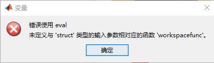
    甚至有的人安装好Matlab以后，什么操作也不做，仅仅是将软件打开就会有这样的报错。

解决方法一：（很多人用这种方法奏效了）
    但对我来说似乎没什么用。

解决方法二：
    先把“设置路径”恢复成默认（之前设置的就没有了，不知道有没有更好的方法），把新的工具箱a解压到toolbox目录下，然后用addpath把toolbox的路径添加到matlab的搜索路径中，最后用which xxx.m来检验是否可以访问里面的xxx.m文件。如果能够显示新设置的路径，则表明报错解决，该工具箱可以使用了。示例如下：

>> addpath E:\MATLAB\R2018a\toolbox

%输入工具箱名称，此时一般会返回该工具箱的说明，也就是mathmodl 
>> help mathmodl路径下content.m中的内容
%在命令行中输入如下，此时会返回mathmodl路径下所有的文件
>> what mathmodl
%再到mathmodl中随便找一个不与Matlab中重名的函数，比如xxx.m，在命令行中输入
>> which xxx.m
E:\MATLAB\rvctools\xxx.m
1
2
3
4
5
6
7
8
9

2.Matlab启动过慢：

    这绝对是困扰我很久的一个问题，一度让我怀疑自己设备有问题（虽然确实慢）。
    如果你的matlab停留在“正在初始化…”这个界面长达几分钟甚至更久，试试下面的方法（据说是最近几代新版本的共性问题）：
    启动慢的原因是软件查找授权文件时间太长，我们定位到license文件，找到license文件的绝对路径（我的就在一级安装文件下），删除这个文件license_server.lic（不同版本的名字是不一样的！大家试一下）。
    剩下的文件如图：

    然后速度瞬间提升了hhh。

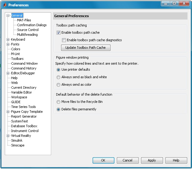
3.Matlab启动的时候给出警告：

Warning: MATLAB Toolbox Path Cache is out of date and is not being used. Type 'help toolbox_path_cache' for more info.To get started, select MATLAB Help or Demos from the Help menu.

    这个问题式因为安装工具箱之后没有更新缓存，解决方法：
    File——>Preferences——>General——>选中enable toolbox path cache——>点击updata toolbox path cache

---

二、使用机器人工具箱创建双足机器人：

1.复现双足机器人：

    原博：JianRobSim

%% 主代码
%% 说明：我用了原博的代码腿的位置不对，troty(-pi/2)改成了troty(pi/2)对了
%% creat walking robot model
clear all
%leg length 
L1=0.15;L2=0.25;
%form a leg 
leg=SerialLink([0, 0, 0, pi/2; 0, 0, L1, 0; 0, 0, -L2, 0 ],...
    'name', 'leg', 'base', eye(4,4),'tool', ...
    troty(pi/2)*trotx(-pi/2)*trotz(-pi/2),'offset', [pi/2  0  -pi/2]);
%% diplay the leg 
%body wide and length
W = 0.2; L = 0.2;
%form a body
legs(1) = SerialLink(leg, 'name', 'leg1','base', transl(0, 0, -0.05)*trotz(pi/2));  %*trotz(pi/2)
legs(2) = SerialLink(leg, 'name', '.', 'base', transl(0, -W, -0.05)*trotz(pi/2));
% create a fixed size axis for the robot, and set z positive downward
clf;
axis([-0.3 0.25 -0.6 0.4 -0.19 0.45]); set(gca,'Zdir', 'reverse')
hold on
legs(1).plot([0 pi/3 -pi/2.5],'nobase','noshadow','nowrist');%leg pose
legs(2).plot([0 pi/1.8 -pi/2.5],'nobase','noshadow','nowrist');
%plot body
plotcube([0.1 0.2 -0.12],[ -0.05  -0.2  0],1,[1 1 0]);
%% simulate moving
for i=0.01:0.02:0.4
legs(1).plot([0   pi/3+i    -pi/2.5-i],'nobase','noshadow');%leg pose
legs(2).plot([0   pi/1.8-i  -pi/2.5+i],'nobase','noshadow');
end
1
2
3
4
5
6
7
8
9
10
11
12
13
14
15
16
17
18
19
20
21
22
23
24
25
26
27
28
29

% 身体控制器
function plotcube(varargin)
% PLOTCUBE - Display a 3D-cube in the current axes
%
%   PLOTCUBE(EDGES,ORIGIN,ALPHA,COLOR) displays a 3D-cube in the current axes
%   with the following properties:
%   * EDGES : 3-elements vector that defines the length of cube edges
%   * ORIGIN: 3-elements vector that defines the start point of the cube
%   * ALPHA : scalar that defines the transparency of the cube faces (from 0
%             to 1)
%   * COLOR : 3-elements vector that defines the faces color of the cube
%
% Example:
%   >> plotcube([5 5 5],[ 2  2  2],.8,[1 0 0]);
%   >> plotcube([5 5 5],[10 10 10],.8,[0 1 0]);
%   >> plotcube([5 5 5],[20 20 20],.8,[0 0 1]);
%% plotcube函数 长宽高  三维空间起点  颜色属性
% Default input arguments
inArgs = { ...
  [10 56 100] , ... % Default edge sizes (x,y and z)
  [10 10  10] , ... % Default coordinates of the origin point of the cube
  .7          , ... % Default alpha value for the cube's faces
  [1 0 0]       ... % Default Color for the cube
  };
 
% Replace default input arguments by input values
inArgs(1:nargin) = varargin;
 
% Create all variables
[edges,origin,alpha,clr] = deal(inArgs{:});
 
XYZ = { ...
  [0 0 0 0]  [0 0 1 1]  [0 1 1 0] ; ...
  [1 1 1 1]  [0 0 1 1]  [0 1 1 0] ; ...
  [0 1 1 0]  [0 0 0 0]  [0 0 1 1] ; ...
  [0 1 1 0]  [1 1 1 1]  [0 0 1 1] ; ...
  [0 1 1 0]  [0 0 1 1]  [0 0 0 0] ; ...
  [0 1 1 0]  [0 0 1 1]  [1 1 1 1]   ...
  };
 
XYZ = mat2cell(...
  cellfun( @(x,y,z) x*y+z , ...
    XYZ , ...
    repmat(mat2cell(edges,1,[1 1 1]),6,1) , ...
    repmat(mat2cell(origin,1,[1 1 1]),6,1) , ...
    'UniformOutput',false), ...
  6,[1 1 1]);
 
 
cellfun(@patch,XYZ{1},XYZ{2},XYZ{3},...
  repmat({clr},6,1),...
  repmat({'FaceAlpha'},6,1),...
  repmat({alpha},6,1)...
  );
 
% view(3);
1
2
3
4
5
6
7
8
9
10
11
12
13
14
15
16
17
18
19
20
21
22
23
24
25
26
27
28
29
30
31
32
33
34
35
36
37
38
39
40
41
42
43
44
45
46
47
48
49
50
51
52
53
54
55
56

    在这个项目的最后，博主贴了一个simscape的仿真结果，确实流畅度高了很多。所以我的下一步学习计划就是simscape~

2.复现机械臂：

    参考博主，具体讲解可以点进去看。

clear ; clc; close all;
% 机器人各连杆DH参数
d1 = 0;
d2 = 86;
d3 = -92;

% 由于关节4为移动关节，故d4为变量，theta4为常量
theta4 = 0;
a1 = 400;
a2 = 250;
a3 = 0;
a4 = 0;

alpha1 = 0 / 180 * pi;
alpha2 = 0 / 180 * pi;
alpha3 = 180 / 180 * pi;
alpha4 = 0 / 180 * pi;

% 定义各个连杆，默认为转动关节
%           theta      d        a        alpha 
L(1)=Link([  0         d1      a1      alpha1]); L(1).qlim=[-pi,pi];
L(2)=Link([  0         d2      a2      alpha2]); L(2).qlim=[-pi,pi]; L(2).offset=pi/2;
L(3)=Link([  0         d3      a3      alpha3]); L(3).qlim=[-pi,pi];

% 移动关节需要特别指定关节类型--jointtype
L(4)=Link([theta4       0      a4      alpha4]); L(4).qlim=[0,180]; L(4).jointtype='P';

% 把上述连杆“串起来”
Scara=SerialLink(L,'name','Scara');

% 定义机器人基坐标和工具坐标的变换
Scara.base = transl(0 ,0 ,305);
Scara.tool = transl(0 ,0 ,100);   
Scara.teach();   %机器人示教界面

% 绘制动画
figure
joint(: , 1) = linspace(pi/6,pi/2,100);
joint(: , 2) = linspace(0,pi/4,100);
joint(: , 3) = linspace(pi/3,pi/2,100);
joint(: , 4) = linspace(0,160,100);
filename = 'demo.gif';
for i = 1:length(joint)
    pause(0.01)
    Scara.plot(joint(i,:));
    f = getframe(gcf);  
    imind = frame2im(f);
    [imind,cm] = rgb2ind(imind,256);
    if i == 1
        imwrite(imind,cm,filename,'gif', 'Loopcount',inf,'DelayTime',0.1);
    else      imwrite(imind,cm,filename,'gif','WriteMode','append','DelayTime',0.1);
    end
end
1
2
3
4
5
6
7
8
9
10
11
12
13
14
15
16
17
18
19
20
21
22
23
24
25
26
27
28
29
30
31
32
33
34
35
36
37
38
39
40
41
42
43
44
45
46
47
48
49
50
51
52
53

    接下来有一个改进DH方法的代码，其实主要是 'modified’参数的改变：

clear ; clc; close all;
% 机器人各连杆参数值
d1 = 670;
d2 = 0;
d3 = 0;
d4 = 1280;
d5 = 0;
d6 = 215;

a1 = 0;
a2 = 312;
a3 = 1075;
a4 = 225;
a5 = 0;
a6 = 0;

alpha1 = 0 / 180 * pi;
alpha2 = -90 / 180 * pi;
alpha3 = 0 / 180 * pi;
alpha4 = -90 / 180 * pi;
alpha5 = 90 / 180 * pi;
alpha6 = -90 / 180 * pi;
% 建立连杆DH参数（修正的DH）
L(1)=Link([0 d1 a1 alpha1], 'modified'); L(1).qlim=[-pi,pi];
L(2)=Link([0 d2 a2 alpha2], 'modified');  L(2).qlim=[-pi,pi];L(2).offset = -pi/2;
L(3)=Link([0 d3 a3 alpha3], 'modified'); L(3).qlim=[-pi,pi];
L(4)=Link([0 d4 a4 alpha4], 'modified'); L(4).qlim=[-pi,pi];
L(5)=Link([0 d5 a5 alpha5], 'modified'); L(5).qlim=[-pi,pi];
L(6)=Link([0 d6 a6 alpha6], 'modified'); L(6).qlim=[-pi,pi];
% 定义机器人
FANUC=SerialLink(L(1:6),'name','FANUC');
FANUC.tool = transl(0,0,100);
FANUC.teach();
1
2
3
4
5
6
7
8
9
10
11
12
13
14
15
16
17
18
19
20
21
22
23
24
25
26
27
28
29
30
31
32
33

    为了搞清楚standard DH和modified DH，我看了好久的资料，简单谈一下我的理解。

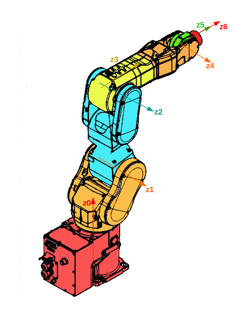
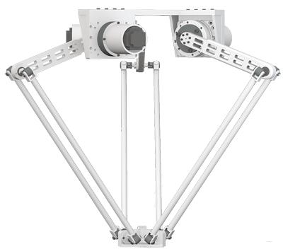
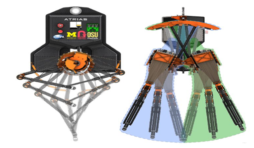
    以这张图（来源）为例，标准DH方法是在传动轴上（远端，如图）建立坐标系的，所以 z 轴（为了避免麻烦，只画z轴）建立在连杆远离基座一侧的那个轴上；改进DH方法则会把坐标系建立在固定轴上（近端）。
    这两种建系方法对于平常的普通机械臂是没有区别的，在matlab里的体现也只是修改“modified”参数的问题，最多是得到的转换矩阵结果不同。但是对于delta、Atrias这样的并联机器人，或者树状、轮式结构机器人来说，在进行逆运算时，如果回推原点大于1个，就会出现混乱。

delta机器人

Atrias机器人