常见的激活函数

激活函数：

激活层的原理是在其他层的输出之后添加非线性激活函数，增加网络的非线性能力，提高神经网络拟合复杂函数的能力。激活函数的选择对神经网络的训练至关重要，常用的激活函数包括Sigmoid函数、Tanh函数、ReLU函数和LeakyReLU等。激活层模拟了生物神经系统的刺激过程，将非线性函数引入进来，从而更加有效地进行特征的表征。在卷积神经网络中的卷积层和全连接层，每一层的输出值在本质上都是输入神经元经过计算加权平均值的结果得到的。由于加权平均是线性运算，经过多个卷积层或全连接层的组合叠加，得到的函数依旧是线性变换函数。因此，为了进一步增强卷积神经网络的表达能力，需要将具有非线性特点的激活函数添加到卷积神经网络的结构之中。下面将介绍一些常见的激活函数

学习内容：

Sigmoid

Sigmoid函数是生物学中常见的S型函数，函数曲线如下图所示。它可以把输入的数变换到0~1之间输出，如果输入时特别小的负数，则输出为0，如果输入是特别大的正数，则输出为1。Sigmoid可以看作非线性激活函数赋予网络非线性区分能力，常用在二分类。

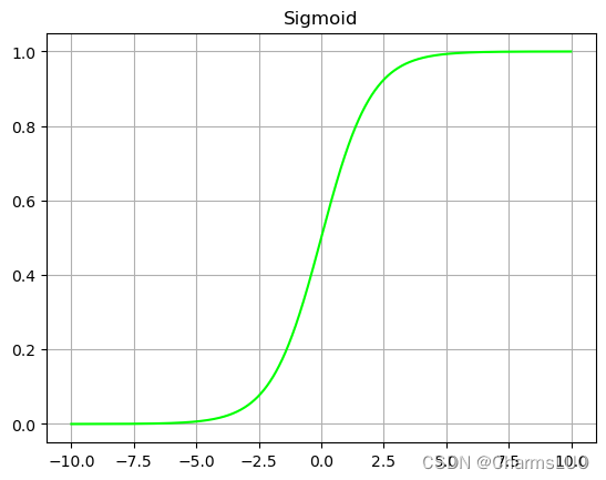
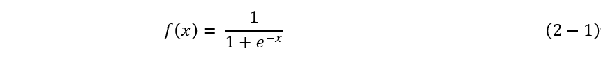
Sigmoid激活函数的计算公式可以表示为公式（2-1），其中x 表示输入的像素。通过分析函数表达式和Sigmoid曲线可以知道，Sigmoid激活函数优点是曲线平滑处处可导；缺点是幂函数运算较慢，激活函数计算量大；求取反向梯度时，Sigmoid的梯度在饱和区域非常平缓，很容易造称梯度消失的问题，减缓收敛速度。

import matplotlib.pyplot as plt
import numpy as np

def Sigmoid(x):
    y = np.exp(x) / (np.exp(x) + 1)
    return y
    
if __name__ == '__main__':

    x = np.arange(-10, 10, 0.01)
    
    plt.plot(x, Sigmoid(x), color = '#00ff00')
    plt.title("Sigmoid")
    plt.grid()
    plt.savefig("Sigmoid.png", bbox_inches='tight')
    plt.show()
1
2
3
4
5
6
7
8
9
10
11
12
13
14
15
16

Tanh

Tanh函数是一个典型的奇函数，函数曲线如下图所示，它能够把输入的连续实值变换为-1和1之间的输出，如果输入是特别小的负数，则输出为-1，如果输入是特别大的正数，则输出为1；解决了Sigmoid函数均值不是0的问题。Tanh可以作为非线性激活函数赋予网络非线性区分能力。

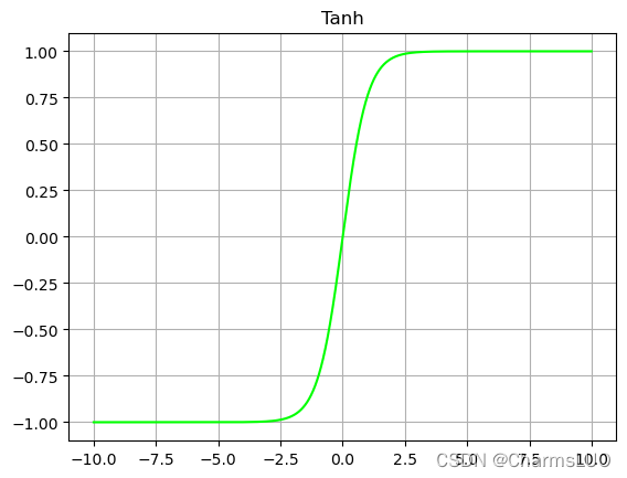
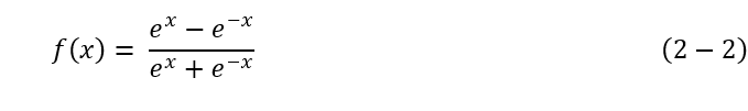
Tanh激活函数的计算公式可以用公式（2-2）表示，其中x 表示输入。通过分析函数表达式和Tanh曲线可以知道，Tanh激活函数优点是曲线平滑，处处可导，具有良好的对称性，网络均值为0。Tanh函数与Sigmoid类似，幂函数运算较慢，激活函数计算量大；求取反向梯度时，Tanh的梯度在饱和区域非常平缓，很容易造称梯度消失的问题，减缓收敛速度。

import matplotlib.pyplot as plt
import numpy as np

def Tanh(x):
    y = (np.exp(x) - np.exp(-x)) / (np.exp(x) + np.exp(-x))
    # y = np.tanh(x)
    return y
    
if __name__ == '__main__':

    x = np.arange(-10, 10, 0.01)
    
    plt.plot(x, Tanh(x), color = '#00ff00')
    plt.title("Tanh")
    plt.grid()
    plt.savefig("Tanh.png", bbox_inches='tight')
    plt.show()  
1
2
3
4
5
6
7
8
9
10
11
12
13
14
15
16
17

ReLU

线性整流激活函数（Rectified Linear Unit, ReLU），是一种深度神经网络中常用的激活函数，ReLU函数曲线如下图所示，整个函数可以分为两部分，在小于0的部分，激活函数的输出为0；在大于0的部分，激活函数的输出为输入。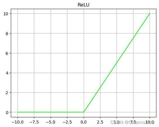

ReLU激活函数的计算公式可以用公式（2-3）表示，其中x 表示输入。通过分析函数表达式和ReLU曲线可以知道，ReLU激活函数优点是收敛速度快，不存在饱和区间，在大于0的部分梯度固定为1，有效解决了Sigmoid中存在的梯度消失的问题。计算速度快，ReLU只需要一个阈值就可以得到激活值，而不用去算一大堆复杂的指数运算，具有类生物性质。ReLU函数的缺点是它在训练时可能会“死掉”。如果一个非常大的梯度经过一个ReLU神经元，更新过参数之后，这个神经元的的值都小于0，此时ReLU再也不会对任何数据有激活现象了。如果这种情况发生，那么从此所有流过这个神经元的梯度将都变成 0。合理设置学习率，会降低这种情况的发生概率。

import matplotlib.pyplot as plt
import numpy as np

def ReLU(x):
    y = np.where(x < 0, 0, x)
    return y
    
if __name__ == '__main__':

    x = np.arange(-10, 10, 0.01)
    
    plt.plot(x, ReLU(x), color = '#00ff00')
    plt.title("ReLU")
    plt.grid()
    plt.savefig("ReLU.png", bbox_inches='tight')
    plt.show()
1
2
3
4
5
6
7
8
9
10
11
12
13
14
15
16

LeakyReLU

LeakyReLU是ReLU函数的改进版，普通的ReLU是将所有的负值都设为零，Leaky ReLU则是给所有负值赋予一个非零斜率，在反向传播过程中，对于LeakyReLU激活函数输入小于零的部分，也可以计算得到梯度.避免了梯度消失问题。LeakyReLU激活函数图像如图2-8所示。

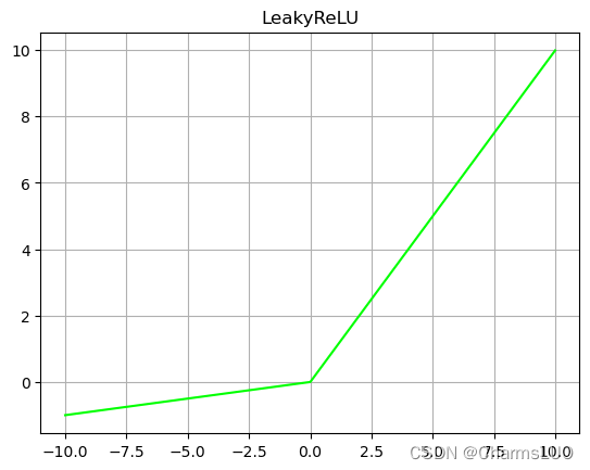
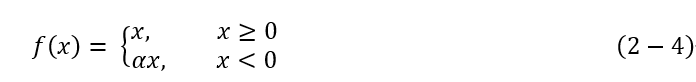
LeakyReLU激活函数的计算公式可以表达为公式为（2-4），其中x 表示输入。通过函数表达式和LeakyReLU曲线可以知道LeakyReLU具有ReLU的优点；解决了ReLU函数存在的问题，防止死亡神经元的出现。缺点是α参数需要人工选择，具体的的值需要根据任务的需要选择。

import matplotlib.pyplot as plt
import numpy as np

def LeakyReLU(x, a):
    # LeakyReLU的a参数不可训练，人为指定。
    y = np.where(x < 0, a * x, x)
    return y
    
if __name__ == '__main__':

    x = np.arange(-10, 10, 0.01)
    
    plt.plot(x, LeakyReLU(x, 0.1), color = '#00ff00')
    plt.title("LeakyReLU")
    plt.grid()
    plt.savefig("LeakyReLU.png", bbox_inches='tight')
    plt.show()
1
2
3
4
5
6
7
8
9
10
11
12
13
14
15
16
17

ELU

ELU激活函数函数曲线如下图所示，输入大于0部分的梯度为1,输入小于0的部分无限趋近于-a。理想的激活函数应满足输出的分布是零均值的，可以加快训练速度。激活函数是单侧饱和的，可以更好的收敛，ELU激活函数同时满足这两个特性。在本文第四张，设计Encoder-Decoder网络中，会使用ELU激活函数。

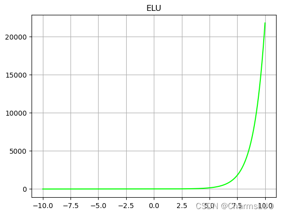
ELU激活函数的计算公式可以表达为公式（2-5），其中x 是输入。通过分析函数表达式和ELU函数曲线可以知道，函数的输出分布式零均值的，因此可以单独使用，在前面可以不用加BN层，ELU函数具有单饱和性，可以更好的收敛。由于ELU牵涉到指数运算，因此推理速度相对耗时。

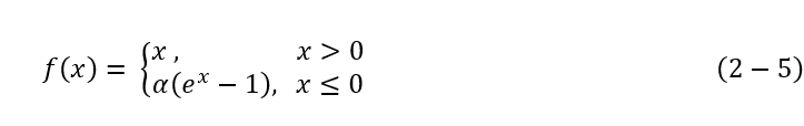
import matplotlib.pyplot as plt
import numpy as np

def ELU(x, a):
    y = np.where(x < 0, x, a*(np.exp(x)-1))
    return y
    
if __name__ == '__main__':

    x = np.arange(-10, 10, 0.01)
    
    plt.plot(x, ELU(x, 1),  color = '#00ff00')
    plt.title("ELU")
    plt.grid()
    plt.savefig("ELU.png", bbox_inches='tight')
    plt.show()
1
2
3
4
5
6
7
8
9
10
11
12
13
14
15
16

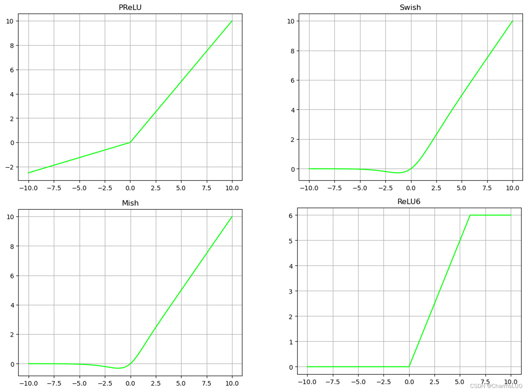
其他激活函数

PReLU、ReLU6、Swish、Mish

其他激活函数都是在上述激活函数的改进下提出来的，代码，我放在下面了

import matplotlib.pyplot as plt
import numpy as np


def Sigmoid(x):
    y = np.exp(x) / (np.exp(x) + 1)
    return y


def Tanh(x):
    y = (np.exp(x) - np.exp(-x)) / (np.exp(x) + np.exp(-x))
    # y = np.tanh(x)
    return y


def ReLU(x):
    y = np.where(x < 0, 0, x)
    return y


def LeakyReLU(x, a):
    # LeakyReLU的a参数不可训练，人为指定。
    y = np.where(x < 0, a * x, x)
    return y

def ELU(x, a):
    y = np.where(x < 0, x, a*(np.exp(x)-1))
    return y


def PReLU(x, a):
    # PReLU的a参数可训练
    y = np.where(x < 0, a * x, x)
    return y


def ReLU6(x):
    y = np.minimum(np.maximum(x, 0), 6)
    return y


def Swish(x, b):
    y = x * (np.exp(b * x) / (np.exp(b * x) + 1))
    return y


def Mish(x):
    # 这里的Mish已经经过e和ln的约运算
    temp = 1 + np.exp(x)
    y = x * ((temp * temp - 1) / (temp * temp + 1))
    return y


def Grad_Swish(x, b):
    y_grad = np.exp(b * x) / (1 + np.exp(b * x)) + x * (b * np.exp(b * x) / ((1 + np.exp(b * x)) * (1 + np.exp(b * x))))
    return y_grad


def Grad_Mish(x):
    temp = 1 + np.exp(x)
    y_grad = (temp * temp - 1) / (temp * temp + 1) + x * (4 * temp * (temp - 1)) / (
                (temp * temp + 1) * (temp * temp + 1))
    return y_grad


if __name__ == '__main__':
    x = np.arange(-10, 10, 0.01)

    plt.plot(x, Sigmoid(x), color = '#00ff00')
    plt.title("Sigmoid")
    plt.grid()
    plt.savefig("Sigmoid.png", bbox_inches='tight')
    plt.show()

    plt.plot(x, Tanh(x), color = '#00ff00')
    plt.title("Tanh")
    plt.grid()
    plt.savefig("Tanh.png", bbox_inches='tight')
    plt.show()

    plt.plot(x, ReLU(x), color = '#00ff00')
    plt.title("ReLU")
    plt.grid()
    plt.savefig("ReLU.png", bbox_inches='tight')
    plt.show()

    plt.plot(x, LeakyReLU(x, 0.1), color = '#00ff00')
    plt.title("LeakyReLU")
    plt.grid()
    plt.savefig("LeakyReLU.png", bbox_inches='tight')
    plt.show()

    plt.plot(x, ELU(x, 1),  color = '#00ff00')
    plt.title("ELU")
    plt.grid()
    plt.savefig("ELU.png", bbox_inches='tight')
    plt.show()

    plt.plot(x, PReLU(x, 0.25), color = '#00ff00')
    plt.title("PReLU")
    plt.grid()
    plt.savefig("PReLU.png", bbox_inches='tight')
    plt.show()

    plt.plot(x, ReLU6(x), color = '#00ff00')
    plt.title("ReLU6")
    plt.grid()
    plt.savefig("ReLU6.png", bbox_inches='tight')
    plt.show()

    plt.plot(x, Swish(x, 1), color = '#00ff00')
    plt.title("Swish")
    plt.grid()
    plt.savefig("Swish.png", bbox_inches='tight')
    plt.show()

    plt.plot(x, Mish(x), color = '#00ff00')
    plt.title("Mish")
    plt.grid()
    plt.savefig("Mish.png", bbox_inches='tight')
    plt.show()


    plt.plot(x, Grad_Mish(x))
    plt.plot(x, Grad_Swish(x, 1))
    plt.title("Gradient of Mish and Swish")
    plt.legend(['Mish', 'Swish'])
    plt.grid()
    plt.savefig("MSwith.png", bbox_inches='tight')
    plt.show()



1
2
3
4
5
6
7
8
9
10
11
12
13
14
15
16
17
18
19
20
21
22
23
24
25
26
27
28
29
30
31
32
33
34
35
36
37
38
39
40
41
42
43
44
45
46
47
48
49
50
51
52
53
54
55
56
57
58
59
60
61
62
63
64
65
66
67
68
69
70
71
72
73
74
75
76
77
78
79
80
81
82
83
84
85
86
87
88
89
90
91
92
93
94
95
96
97
98
99
100
101
102
103
104
105
106
107
108
109
110
111
112
113
114
115
116
117
118
119
120
121
122
123
124
125
126
127
128
129
130
131
132
133