rrt* 算法_rrt*算法

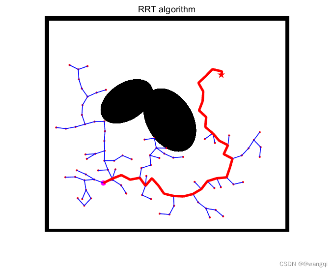
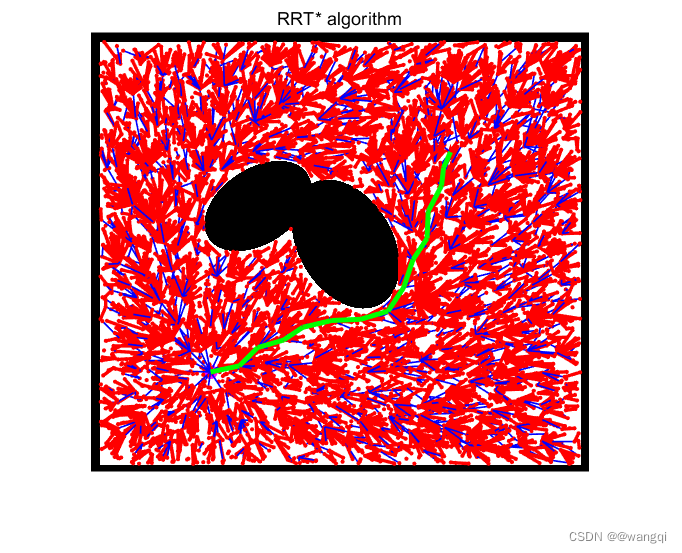
  rrt算法由于没有考虑cost值，使得最终规划的路径质量很差。rrt*算法在此基础上，引入贪心思想，使得规划路径可以随着采样次数增多逐步优化。

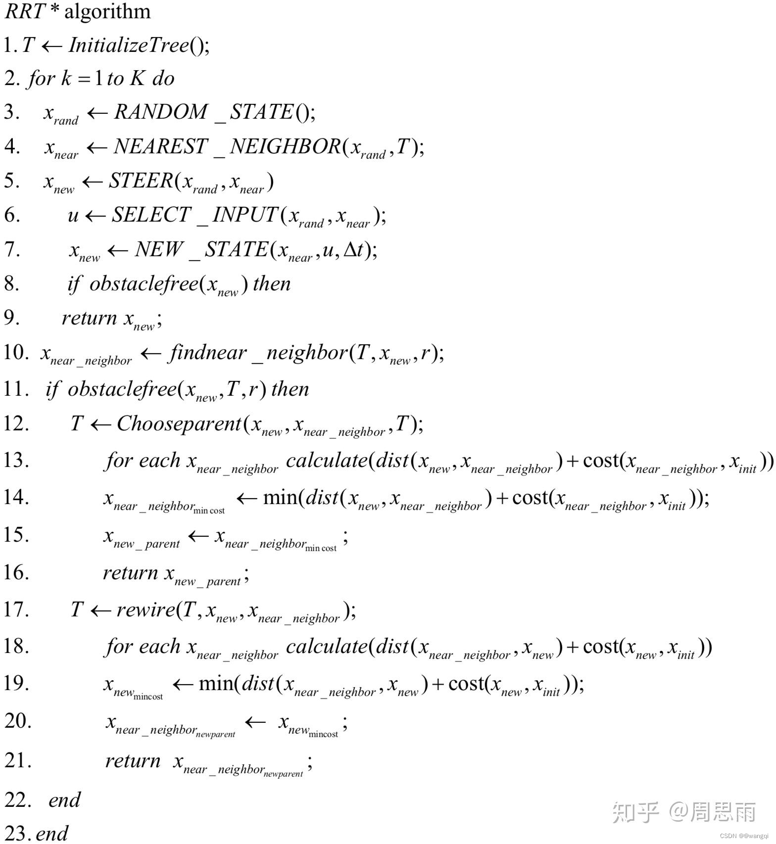
一、算法流程

二、rrt*与rrt的不同

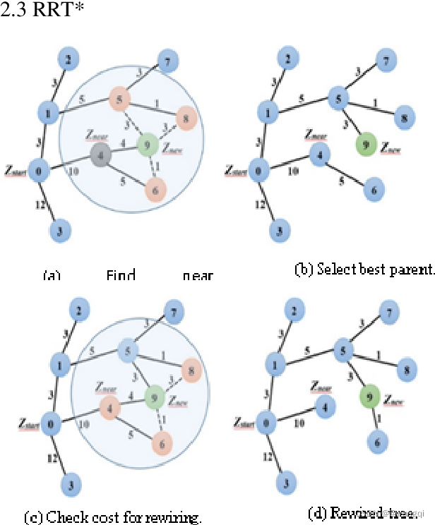
1、父节点的选取不同

        rrt扩展完后，将距离其最近的节点作为其父节点；而rrt*是划定一个范围，将范围的节点均作为待选父节点，然后分别计算以它们为父节点时，的cost值，选择使的cost最小的节点作为其父节点。这一步使得扩展得新节点得cost尽可能得小。

2、重布线（rewire）

        在完成新节点的父节点选取后，选取新节点的周边节点，假设将刚扩展的新节点作为它们的父节点，比较此时它们的cost值与其原先得cost值，如果此时cost值较小，则rewire，将新节点作为其父节点，并更新cost值。

三、matlab代码

这里只放两处关键代码，后面会上传github。

1、父节点的选取

%以newnode节点为中心，半径R为半径搜索节点
R=30/ceil(0.001*numel(nodes_list));
dis2new=nodes_list(ind).cost+stepLength;
minCostIndex=ind;
nearNodeList=[];
for index_near=1:N
    if norm(nodes_list(index_near).position-newnode)<R
        nearNodeList=[nearNodeList,nodes_list(index_near)]; %if node in the range, put it in the nearNodeList
        if norm(nodes_list(index_near).position-newnode)+nodes_list(index_near).cost<dis2new
            dis2new=norm(nodes_list(index_near).position-newnode)+nodes_list(index_near).cost;
            flag=collisionCheck(newnode,nodes_list(index_near).position,fig);
            if flag
                minCostIndex=index_near;
            end
        end
    end
end
lhandle=plot([nodes_list(minCostIndex).position(1),newnode(1)],[nodes_list(minCostIndex).position(2),newnode(2)],'b-','LineWidth',1);
lhandlelist=[lhandlelist,lhandle];
phandle=plot(newnode(1),newnode(2),'ro','MarkerFaceColor','r','MarkerSize',2);
phandlelist=[phandlelist,phandle];
drawnow;
nodes_list(N+1).position=newnode;
nodes_list(N+1).parentind=minCostIndex;
nodes_list(N+1).cost=nodes_list(minCostIndex).cost+norm(near2rand);
nodes_list(N+1).index=N+1;

2、rewire

%% rewire
NearNums=length(nearNodeList);
for iterNear=1:NearNums
    nearNewCost=norm(nearNodeList(iterNear).position-newnode);
    if nearNewCost+nodes_list(N+1).cost<nearNodeList(iterNear).cost
        flag=collisionCheck(newnode,nearNodeList(iterNear).position,fig);
        if flag
            nodes_list(nearNodeList(iterNear).index).parentind=N+1;
            nodes_list(nearNodeList(iterNear).index).cost=nearNewCost+nodes_list(N+1).cost;
            %delete(lhandlelist(nearNodeList(iterNear).index-1));
            lhandlelist(nearNodeList(iterNear).index-1)=plot([nearNodeList(iterNear).position(1),newnode(1)],...
                [nearNodeList(iterNear).position(2),newnode(2)],'r-','LineWidth',2);
            drawnow;
        end
    end
end
if norm(newnode-goalPoint)<=stepLength && ~findflag
    findflag=1;
    nodes_list(N+2).position=goalPoint;
    nodes_list(N+2).parentind=N+1;
    nodes_list(N+2).cost=nodes_list(N+1).cost+norm(newnode-goalPoint);
    nodes_list(N+2).index=N+2;
    goalindex=N+2;
    %plot([newnode(1),goalPoint(1)],[newnode(2),goalPoint(2)],'b-');
end
title(['RRT* algorithm ','sampleNums:',num2str(j)]);
if findflag
    updatepathcount=updatepathcount+1;
    if updatepathcount==50
        updatepathcount=0;
        m=2;
        path=[];
        path(1).position=goalPoint;
        pathIndex=nodes_list(goalindex).parentind;
        while 1
            path(m).position = nodes_list(pathIndex).position;
            pathIndex = nodes_list(pathIndex).parentind;    % 沿终点回溯到起点
            if pathIndex == -1
                break
            end
            m=m+1;
        end
        for delete_index=1:length(pathhandlelist)
            delete(pathhandlelist(delete_index));
        end
        for m=2:length(path)
            pathhandle=plot([path(m).position(1),path(m-1).position(1)],[path(m).position(2),path(m-1).position(2)],'g-','LineWidth',3);
            pathhandlelist=[pathhandlelist,pathhandle];
        end
    end
end

四、几点疑问 

 1、采样次数与时间复杂度的取舍，采样次数越多，路线越优化。

2、随着采样次数增多，后期的父节点选取及rewire的待选节点越多，这一点如何处理。(有人把搜索半径与采样次数关联，采样次数越多，搜索半径越小）。

3、搜索半径的问题，同样半径越大，路径会越优化，但会带来时间成本的增大。

五、参考文章

http://路径规划——改进RRT算法 - 搬砖的旺财的文章 - 知乎 https://zhuanlan.zhihu.com/p/51087819