学习率衰减方法

目录

指数衰减

固定值衰减

按步长衰减

给定值衰减

---

优化器优化的是学习率，他发生在反向运算中。学习率衰减，是每次迭代衰减的方法，在前向运算中。

学习率设定思路是前期一个较大的学习率来确保加速收敛，后期用较小的学习率保证稳定。一般都是0.01,0.005,0.0001等等之类的，设置初始值。

指数衰减

 

 

固定值衰减

 

按步长衰减

 

$lr = lr_{base} \cdot \tau ^{|\frac{step}{stepsize}|}$

$lr_{base}$基础学习率。$\tau$小于1衰减率。stepsize是个阈值，当前迭代步伐step除以他，向下取整作为$\tau$的指数。衰减系数和stepsize都是经验值。

给定值衰减

facenet中有个文件 ，设定迭代多少次用某个学习率。

 

还有按倒数衰减，按多项式衰减，都需要经验系数来确定，如果经验不足，可以设置自适应。

---

学习率衰减 总结

				版权声明：本文为博主原创文章，未经博主允许不得转载。					https://blog.csdn.net/akadiao/article/details/79560731				</div>
							<link rel="stylesheet" href="https://csdnimg.cn/release/phoenix/template/css/ck_htmledit_views-f57960eb32.css">
							            <div id="content_views" class="markdown_views">
						<!-- flowchart 箭头图标 勿删 -->
						<svg xmlns="http://www.w3.org/2000/svg" style="display: none;"><path stroke-linecap="round" d="M5,0 0,2.5 5,5z" id="raphael-marker-block" style="-webkit-tap-highlight-color: rgba(0, 0, 0, 0);"></path></svg>
						<h3 id="学习率衰减"><a name="t0"></a>学习率衰减</h3>

学习率衰减（learning rate decay）
在训练神经网络时，使用学习率控制参数的更新速度．学习率较小时，会大大降低参数的更新速度；学习率较大时，会使搜索过程中发生震荡，导致参数在极优值附近徘徊．
为此，在训练过程中引入学习率衰减，使学习率随着训练的进行逐渐衰减．

TensorFlow中实现的学习率衰减方法：

• tf.train.piecewise_constant　分段常数衰减
• tf.train.inverse_time_decay　反时限衰减
• tf.train.polynomial_decay　多项式衰减
• tf.train.exponential_decay　指数衰减
• tf.train.natural_exp_decay　自然指数衰减
• tf.train.cosine_decay　余弦衰减
• tf.train.linear_cosine_decay　线性余弦衰减
• tf.train.noisy_linear_cosine_decay　噪声线性余弦衰减
  函数返回衰减的学习率．

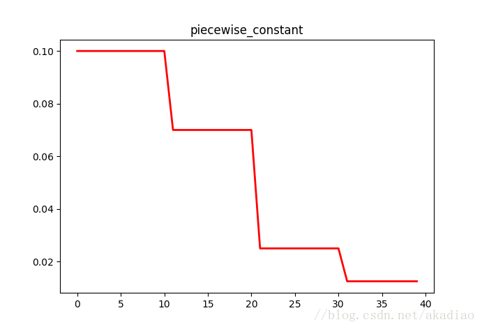
分段常数衰减

tf.train.piecewise_constant()　指定间隔的分段常数．
参数：

• x：0-D标量Tensor．
• boundaries：边界，tensor或list.
• values：指定定义区间的值．
• name：操作的名称，默认为PiecewiseConstant．

分段常数衰减就是在定义好的区间上，分别设置不同的常数值，作为学习率的初始值和后续衰减的取值．

示例：

#!/usr/bin/python
# coding:utf-8
 
# piecewise_constant 阶梯式下降法
import matplotlib.pyplot as plt
import tensorflow as tf
global_step = tf.Variable(0, name='global_step', trainable=False)
boundaries = [10, 20, 30]
learing_rates = [0.1, 0.07, 0.025, 0.0125]
y = []
N = 40
with tf.Session() as sess:
    sess.run(tf.global_variables_initializer())
    for global_step in range(N):
        learing_rate = tf.train.piecewise_constant(global_step, boundaries=boundaries, values=learing_rates)
        lr = sess.run([learing_rate])
        y.append(lr[0])
 
x = range(N)
plt.plot(x, y, 'r-', linewidth=2)
plt.title('piecewise_constant')
plt.show()

 

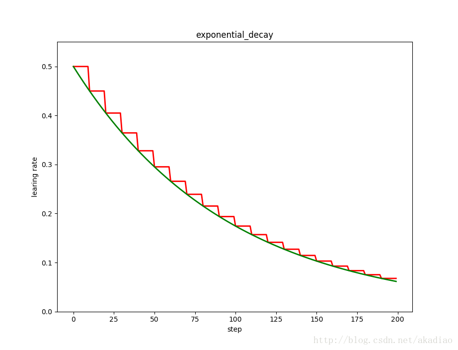
指数衰减

指数衰减

tf.train.exponential_decay()　应用指数衰减的学习率．
指数衰减是最常用的衰减方法．
参数：

• learning_rate：初始学习率．
• global_step：用于衰减计算的全局步数，非负．用于逐步计算衰减指数．
• decay_steps：衰减步数，必须是正值．决定衰减周期．
• decay_rate：衰减率．
• staircase：若为True，则以不连续的间隔衰减学习速率即阶梯型衰减（就是在一段时间内或相同的eproch内保持相同的学习率）；若为False，则是标准指数型衰减．
• name：操作的名称，默认为ExponentialDecay．（可选项）

指数衰减的学习速率计算公式为：

decayed_learning_rate = learning_rate * decay_rate ^ (global_step / decay_steps)  

 

优点：简单直接，收敛速度快．

示例，阶梯型衰减与指数型衰减对比：

#!/usr/bin/python
# coding:utf-8
import matplotlib.pyplot as plt
import tensorflow as tf
global_step = tf.Variable(0, name='global_step', trainable=False)
 
y = []
z = []
N = 200
with tf.Session() as sess:
    sess.run(tf.global_variables_initializer())
    for global_step in range(N):
        # 阶梯型衰减
        learing_rate1 = tf.train.exponential_decay(
            learning_rate=0.5, global_step=global_step, decay_steps=10, decay_rate=0.9, staircase=True)
        # 标准指数型衰减
        learing_rate2 = tf.train.exponential_decay(
            learning_rate=0.5, global_step=global_step, decay_steps=10, decay_rate=0.9, staircase=False)
        lr1 = sess.run([learing_rate1])
        lr2 = sess.run([learing_rate2])
        y.append(lr1[0])
        z.append(lr2[0])
 
x = range(N)
fig = plt.figure()
ax = fig.add_subplot(111)
ax.set_ylim([0, 0.55])
plt.plot(x, y, 'r-', linewidth=2)
plt.plot(x, z, 'g-', linewidth=2)
plt.title('exponential_decay')
ax.set_xlabel('step')
ax.set_ylabel('learing rate')
plt.show()

 

如图，红色：阶梯型；绿色：指数型：

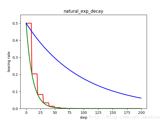
自然指数衰减

tf.train.natural_exp_decay() 　应用自然指数衰减的学习率．
参数：

• learning_rate：初始学习率．
• global_step：用于衰减计算的全局步数，非负.
• decay_steps：衰减步数．
• decay_rate：衰减率．
• staircase：若为True，则是离散的阶梯型衰减（就是在一段时间内或相同的eproch内保持相同的学习率）；若为False，则是标准型衰减．
• name: 操作的名称，默认为ExponentialTimeDecay．

natural_exp_decay 和 exponential_decay 形式近似，natural_exp_decay的底数是e．自然指数衰减比指数衰减要快的多，一般用于较快收敛，容易训练的网络．
自然指数衰减的学习率计算公式为：

decayed_learning_rate = learning_rate * exp(-decay_rate * global_step)

 

示例，指数衰减与自然指数衰减的阶梯型与指数型：

#!/usr/bin/python
# coding:utf-8
 
import matplotlib.pyplot as plt
import tensorflow as tf
global_step = tf.Variable(0, name='global_step', trainable=False)
 
y = []
z = []
w = []
N = 200
with tf.Session() as sess:
    sess.run(tf.global_variables_initializer())
    for global_step in range(N):
        # 阶梯型衰减
        learing_rate1 = tf.train.natural_exp_decay(
            learning_rate=0.5, global_step=global_step, decay_steps=10, decay_rate=0.9, staircase=True)
        # 标准指数型衰减
        learing_rate2 = tf.train.natural_exp_decay(
            learning_rate=0.5, global_step=global_step, decay_steps=10, decay_rate=0.9, staircase=False)
        # 指数衰减
        learing_rate3 = tf.train.exponential_decay(
            learning_rate=0.5, global_step=global_step, decay_steps=10, decay_rate=0.9, staircase=False)
        lr1 = sess.run([learing_rate1])
        lr2 = sess.run([learing_rate2])
        lr3 = sess.run([learing_rate3])
        y.append(lr1[0])
        z.append(lr2[0])
        w.append(lr3[0])
 
x = range(N)
fig = plt.figure()
ax = fig.add_subplot(111)
ax.set_ylim([0, 0.55])
plt.plot(x, y, 'r-', linewidth=2)
plt.plot(x, z, 'g-', linewidth=2)
plt.plot(x, w, 'b-', linewidth=2)
plt.title('natural_exp_decay')
ax.set_xlabel('step')
ax.set_ylabel('learing rate')
plt.show()

 

如图，红色：阶梯型；绿色：指数型；蓝色指数型衰减：

多项式衰减

tf.train.polynomial_decay()　应用多项式衰减的学习率．
参数：

• learning_rate：初始学习率．
• global_step：用于衰减计算的全局步数，非负.
• decay_steps：衰减步数，必须是正值．
• end_learning_rate：最低的最终学习率．
• power：多项式的幂，默认为1.0（线性）．
• cycle：学习率下降后是否重新上升．
• name：操作的名称，默认为PolynomialDecay。

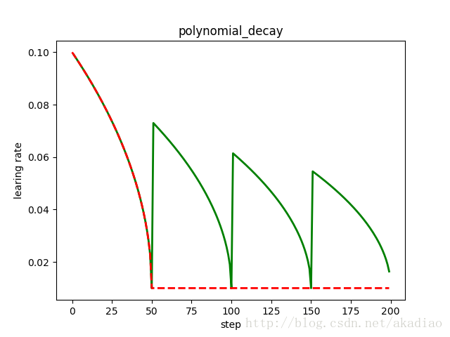
函数使用多项式衰减，以给定的decay_steps将初始学习率（learning_rate）衰减至指定的学习率（end_learning_rate）．

多项式衰减的学习率计算公式为：

global_step = min(global_step,decay_steps)
decayed_learning_rate = (learning_rate-end_learning_rate)*(1-global_step/decay_steps)^ (power)+end_learning_rate

 

参数cycle决定学习率是否在下降后重新上升．若cycle为True，则学习率下降后重新上升；使用decay_steps的倍数，取第一个大于global_steps的结果．

decay_steps = decay_steps*ceil(global_step/decay_steps)
decayed_learning_rate = (learning_rate-end_learning_rate)*(1-global_step/decay_steps)^ (power)+end_learning_rate

参数cycle目的：防止神经网络训练后期学习率过小导致网络一直在某个局部最小值中振荡；这样，通过增大学习率可以跳出局部极小值．

示例，学习率下降后是否重新上升对比：

#!/usr/bin/python
# coding:utf-8
# 学习率下降后是否重新上升
import matplotlib.pyplot as plt
import tensorflow as tf
y = []
z = []
N = 200
global_step = tf.Variable(0, name='global_step', trainable=False)
 
with tf.Session() as sess:
    sess.run(tf.global_variables_initializer())
    for global_step in range(N):
        # cycle=False
        learing_rate1 = tf.train.polynomial_decay(
            learning_rate=0.1, global_step=global_step, decay_steps=50,
            end_learning_rate=0.01, power=0.5, cycle=False)
        # cycle=True
        learing_rate2 = tf.train.polynomial_decay(
            learning_rate=0.1, global_step=global_step, decay_steps=50,
            end_learning_rate=0.01, power=0.5, cycle=True)
        lr1 = sess.run([learing_rate1])
        lr2 = sess.run([learing_rate2])
        y.append(lr1[0])
        z.append(lr2[0])
 
x = range(N)
fig = plt.figure()
ax = fig.add_subplot(111)
plt.plot(x, z, 'g-', linewidth=2)
plt.plot(x, y, 'r--', linewidth=2)
plt.title('polynomial_decay')
ax.set_xlabel('step')
ax.set_ylabel('learing rate')
plt.show()

 

如图，红色：下降后不再上升；绿色：下降后重新上升：

余弦衰减

余弦衰减

tf.train.cosine_decay()　将余弦衰减应用于学习率
参数：

• learning_rate：标初始学习率．
• global_step：用于衰减计算的全局步数.
• decay_steps：衰减步数．
• alpha：最小学习率（learning_rate的部分）。
• name：操作的名称，默认为CosineDecay．

根据论文SGDR: Stochastic Gradient Descent with Warm Restarts提出．

余弦衰减的学习率计算公式为：

global_step = min(global_step, decay_steps)
cosine_decay = 0.5 * (1 + cos(pi * global_step / decay_steps))
decayed = (1 - alpha) * cosine_decay + alpha
decayed_learning_rate = learning_rate * decayed

 

线性余弦衰减

tf.train.linear_cosine_decay()　将线性余弦衰减应用于学习率．
参数：

• learning_rate：标初始学习率．
• global_step：用于衰减计算的全局步数.
• decay_steps：衰减步数。
• num_periods：衰减余弦部分的周期数．
• alpha：见计算．
• beta：见计算．
• name：操作的名称，默认为LinearCosineDecay。

根据论文Neural Optimizer Search with Reinforcement Learning提出．

线性余弦衰减的学习率计算公式为：

global_step=min(global_step,decay_steps)
linear_decay=(decay_steps-global_step)/decay_steps)
cosine_decay = 0.5*(1+cos(pi*2*num_periods*global_step/decay_steps))
decayed=(alpha+linear_decay)*cosine_decay+beta
decayed_learning_rate=learning_rate*decayed

 

噪声线性余弦衰减

tf.train.noisy_linear_cosine_decay()　将噪声线性余弦衰减应用于学习率．
参数：

• learning_rate：标初始学习率．
• global_step：用于衰减计算的全局步数.
• decay_steps：衰减步数．
• initial_variance：噪声的初始方差．
• variance_decay：衰减噪声的方差．
• num_periods：衰减余弦部分的周期数．
• alpha：见计算．
• beta：见计算．
• name：操作的名称，默认为NoisyLinearCosineDecay．

根据论文Neural Optimizer Search with Reinforcement Learning提出．在衰减过程中加入了噪声，一定程度上增加了线性余弦衰减的随机性和可能性．

噪声线性余弦衰减的学习率计算公式为：

global_step=min(global_step,decay_steps)
linear_decay=(decay_steps-global_step)/decay_steps)
cosine_decay=0.5*(1+cos(pi*2*num_periods*global_step/decay_steps))
decayed=(alpha+linear_decay+eps_t)*cosine_decay+beta
decayed_learning_rate =learning_rate*decayed

 

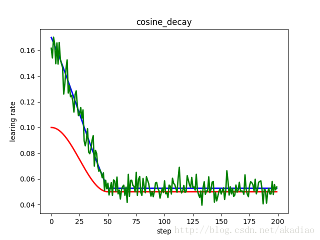
示例，线性余弦衰减与噪声线性余弦衰减：

#!/usr/bin/python
# coding:utf-8
import matplotlib.pyplot as plt
import tensorflow as tf
y = []
z = []
w = []
N = 200
global_step = tf.Variable(0, name='global_step', trainable=False)
 
with tf.Session() as sess:
    sess.run(tf.global_variables_initializer())
    for global_step in range(N):
        # 余弦衰减
        learing_rate1 = tf.train.cosine_decay(
            learning_rate=0.1, global_step=global_step, decay_steps=50,
            alpha=0.5)
        # 线性余弦衰减
        learing_rate2 = tf.train.linear_cosine_decay(
            learning_rate=0.1, global_step=global_step, decay_steps=50,
            num_periods=0.2, alpha=0.5, beta=0.2)
        # 噪声线性余弦衰减
        learing_rate3 = tf.train.noisy_linear_cosine_decay(
            learning_rate=0.1, global_step=global_step, decay_steps=50,
            initial_variance=0.01, variance_decay=0.1, num_periods=0.2, alpha=0.5, beta=0.2)
        lr1 = sess.run([learing_rate1])
        lr2 = sess.run([learing_rate2])
        lr3 = sess.run([learing_rate3])
        y.append(lr1[0])
        z.append(lr2[0])
        w.append(lr3[0])
 
x = range(N)
fig = plt.figure()
ax = fig.add_subplot(111)
plt.plot(x, z, 'b-', linewidth=2)
plt.plot(x, y, 'r-', linewidth=2)
plt.plot(x, w, 'g-', linewidth=2)
plt.title('cosine_decay')
ax.set_xlabel('step')
ax.set_ylabel('learing rate')
plt.show()

 

如图，红色：余弦衰减；蓝色：线性余弦衰减；绿色：噪声线性余弦衰减；

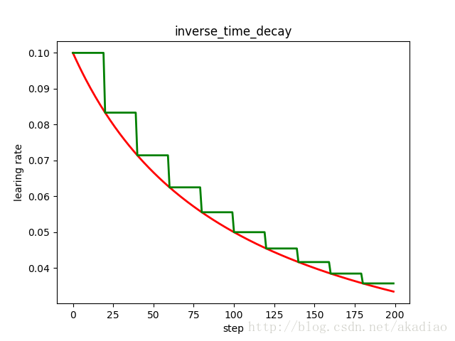
反时限衰减

tf.train.inverse_time_decay()　将反时限衰减应用到初始学习率．
参数：

• learning_rate：初始学习率．
• global_step：用于衰减计算的全局步数．
• decay_steps：衰减步数．
• decay_rate：衰减率．
• staircase：是否应用离散阶梯型衰减．（否则为连续型）
• name：操作的名称，默认为InverseTimeDecay．

该函数应用反向衰减函数提供初始学习速率．利用global_step来计算衰减的学习速率．计算公式为：

decayed_learning_rate =learning_rate/(1+decay_rate* global_step/decay_step)

 

若staircase为True时：

decayed_learning_rate =learning_rate/(1+decay_rate*floor(global_step/decay_step))

 

示例，反时限衰减的阶梯型衰减与连续型对比：

#!/usr/bin/python
# coding:utf-8
 
import matplotlib.pyplot as plt
import tensorflow as tf
y = []
z = []
N = 200
global_step = tf.Variable(0, name='global_step', trainable=False)
 
with tf.Session() as sess:
    sess.run(tf.global_variables_initializer())
    for global_step in range(N):
        # 阶梯型衰减
        learing_rate1 = tf.train.inverse_time_decay(
            learning_rate=0.1, global_step=global_step, decay_steps=20,
            decay_rate=0.2, staircase=True)
        # 连续型衰减
        learing_rate2 = tf.train.inverse_time_decay(
            learning_rate=0.1, global_step=global_step, decay_steps=20,
            decay_rate=0.2, staircase=False)
        lr1 = sess.run([learing_rate1])
        lr2 = sess.run([learing_rate2])
 
        y.append(lr1[0])
        z.append(lr2[0])
 
x = range(N)
fig = plt.figure()
ax = fig.add_subplot(111)
plt.plot(x, z, 'r-', linewidth=2)
plt.plot(x, y, 'g-', linewidth=2)
plt.title('inverse_time_decay')
ax.set_xlabel('step')
ax.set_ylabel('learing rate')
plt.show()

 

如图，蓝色：阶梯型；红色：连续型：