Python绘制nino指数IEP和ICP学习笔记_怎么计算nino3指数

一、数据下载

# 文件地址：https://psl.noaa.gov/data/gridded/data.noaa.ersst.v4.html

厄尔尼诺/拉尼娜事件的主要监测关键区，包括NINO1+2区（90°W-80°W，10°S-0°）、
NINO3区（150°W-90°W，5°S-5°N）、NINO4区（160°E-150°W，5°S-5°N）
和NINO3.4区（170°W-120°W，5°S-5°N）。

承上一篇文章

NINO3.4的3个月滑动平均绝对值达到或超过0.5℃、持续至少5个月，判定为一次厄尔尼诺/拉尼娜事件（指数≥0.5℃为厄尔尼诺事件；指数≤-0.5℃为拉尼娜事件）；以NINO3.4满足事件判定的时间为持续时间。
在事件过程中，NINO3.4的3个月滑动平均绝对值达到最大的时间和数值分别定义为事件的峰值时间和峰值强度。然后，用 IEP和 ICP来判定事件的类型：事件过程中 
IEP的绝对值达到或超过0.5℃且持续至少3个月的类型判定为东部型事件；事件过程中 
ICP的绝对值达到或超过0.5℃且持续至少3个月的类型判定为中部型事件。
若一次事件中同时包含上述两种情况、存在两种类型间的转换，则将事件峰值所在类型定义为事件主体类型，另一种为非主体类型，整个事件的类型以事件主体类型为准。

计算ICP和IEP

IEP=Inino3-α*Inino4

ICP=Inino4-α*Inino3

若nino3*nino4>0.4,α=0.4，否则为0

二、数据处理和绘图

# 导入库
import numpy as np
import matplotlib.pyplot as plt
import netCDF4 as nc
# 设置中英文字体
from matplotlib import rcParams
config = {
    "font.family":'serif',
    "font.size": 14,
    "mathtext.fontset":'stix',
    "font.serif": ['Times New Roman']}
rcParams.update(config)
# 需要加载的数据集
path= r"E:\sst.mnmean.v3.nc" # 1854.01-2020.02年的月均sst
# time<1994> 1994/12=166，即每月测量的平均气温，总共有1994个月，精度为2°
f= nc.Dataset(path)
nsst1=f.variables['sst'][1512:-1,42:47,105:136]#1980-2020
nsst1_3 = f.variables['sst'][1512:1884,42:47,105:136]#1980-2010-NINO3平均海温
nsst2=f.variables['sst'][1512:-1,42:47,80:106]#1980-2020
nsst2_4 = f.variables['sst'][1512:1884,42:47,80:106]#1980-2010-NINO4平均海温
#计算参考https://northfar.net/nino-intro/
#计算多年每个月的平均海温
#Nino3区域
list1=[]
for i in range(0,12):
    a = np.mean(nsst1_3[i:-1:12,:,:],axis=0)
    list1.append(a)
#Nino4区域
list2=[]
for i in range(0,12):
    a = np.mean(nsst2_4[i:-1:12,:,:],axis=0)
    list2.append(a)
# 将每个月的平均海温从nsst中减去
#Nino3区域
anomalies1 = nsst1.copy()
for i in range(0, 12):
    anomalies1[i:-1:12, :, :] -= list1[i]
#Nino4区域
anomalies2 = nsst2.copy()
for i in range(0, 12):
    anomalies2[i:-1:12, :, :] -= list2[i]
 
#计算区域平均nino3.4指数
a1 = np.mean(anomalies1, axis=(1, 2))
a1 = a1[:-1]
a2 = np.mean(anomalies2, axis=(1, 2))
a2 = a2[:-1]
# 根据条件计算a
condition = a1 * a2 > 0.4
a_3 = np.where(condition, a1, a1 - a2 * 0.4)#IEP
a_4 = np.where(condition, a2, a2 - a1 * 0.4)#ICP
 
time = np.arange(1980 , 2020, 1/12)  # 修改这里，确保与数据的时间范围一致
#绘图
# 创建两个子图
fig, (ax, bx) = plt.subplots(2, 1, figsize=(20, 15))
 
# 在第一个子图(ax)上绘制IEP
ax.plot(time, a_3, 'black', alpha=1, linewidth=2)
ax.fill_between(time, 0, a_3, a_3 > 0, color='red', alpha=0.75)
ax.fill_between(time, 0, a_3, a_3 < 0, color='blue', alpha=0.75)
ax.set_ylabel('IEP [$^oC$]')
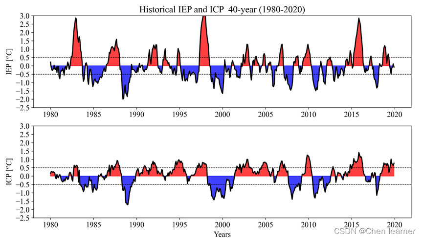
ax.set_title('Historical IEP and ICP  40-year (1980-2020)')
 
# 在第二个子图(bx)上绘制ICP
bx.plot(time, a_4, 'k', alpha=1, linewidth=2)
bx.fill_between(time, 0, a_4, a_4 > 0, color='red', alpha=0.75)
bx.fill_between(time, 0, a_4, a_4 < 0, color='blue', alpha=0.75)
bx.set_xlabel('Years')
bx.set_ylabel('ICP [$^oC$]')
 
# 设置 y 轴范围和刻度间隔
ax.set_ylim(-2.5, 3)
ax.set_yticks(np.arange(-2.5, 3.5, 0.5))
bx.set_ylim(-2.5, 3)
bx.set_yticks(np.arange(-2.5, 3.5, 0.5))
 
# 添加水平虚线
ax.axhline(y=0.5, c='k', lw=0.8, ls='--')
ax.axhline(y=-0.5, c='k', lw=0.8, ls='--')
bx.axhline(y=0.5, c='k', lw=0.8, ls='--')
bx.axhline(y=-0.5, c='k', lw=0.8, ls='--')
# 显示图形
plt.show()

结果如下