盐析白兔

这个屌丝很懒，什么也没留下！

热门标签

自然语言处理—RNN循环神经网络_self.rnn

作者：盐析白兔 | 2024-04-04 15:53:18

踩

self.rnn

1. RNN基本介绍

(参见吴恩达深度学习—RNN篇https://www.bilibili.com/video/BV16r4y1Y7jv?p=152&spm_id_from=pageDriver)

1.1 基本介绍

RNN神经网络可以用来处理时间序列类型的数据，一段文字也可以看成一个时间序列。比如，

The cat ate many food that was delicious was full

$x^{(i)<1>}$ $x^{(i)<2>}$ $x^{(i)<3>}$ $\cdots$ $x^{(i)<t>}$ $\cdots$ $x^{(i)<T_{x}>}$

其中，上标 $i$ 代表第 $(i)$ 个样本， $<t>$ 代表时间，下面将不再样本的标记 $(i)$ 进行分析。一般的神经网络处理时间序列时存在两个问题：i) 输入维度不确定，且如果是one-hot编码，则向量维度高；ii) 一般神经网络不能捕捉序列之间的信息。因此，有循环神经网络来处理时间序列数据。

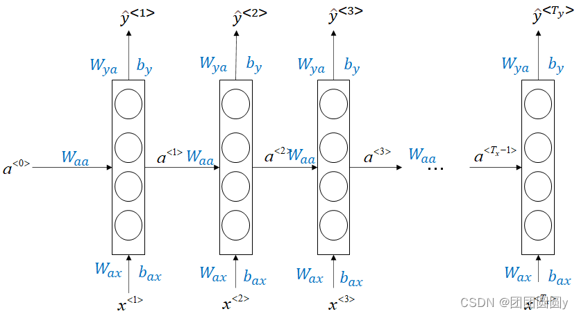
图1. RNN神经网络模型结果

前向传播

在RNN中，每一时刻 $t$ 所使用的参数 $W_{ax}$ 、 $W_{ya}$ 、 $W_{aa}$ 以及 $b_{ax}$ 、 $b_{aa}$ 、 $b_{ya}$ 都是一致的。模型的forward-propagation如下：

$a^{t} = tanh(W_{a}\begin{bmatrix} a^{t-1}\\ x^{t} \end{bmatrix} + b_{a})$

$y^{t} = tanh(W_{y} a^{t}+ b_{y})$ （1）

其中， $W_{a}=\begin{bmatrix} W_{aa} & W_{ax} \end{bmatrix}$ 。

反向传播

每一个时刻，都有损失函数：

$L^{<t>}(y^{t}, \hat{y}^{t}) = -y^{t}log(\hat{y}^{t})-(1-y^{t})log(1-\hat{y}^{t})$

总的损失为 $L = \sum_{t} L^{<t>}$ 。其back-propagation如下图所示，

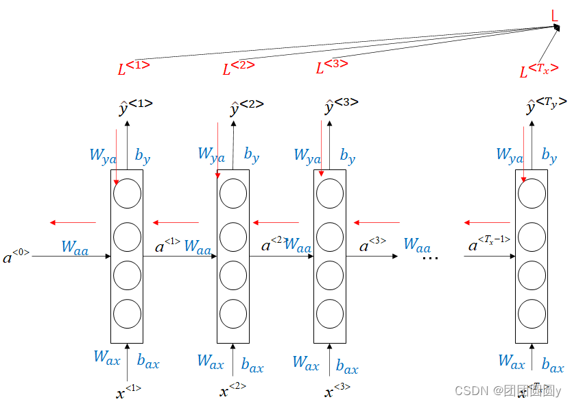
图2. RNN反向传播示意图

上面展示的是 $T_{x} = T_{y}$ 的情形，即输入和输出一样多，根据 $T_{x}$ 和 $T_{y}$ ，有以下多种网络形式。

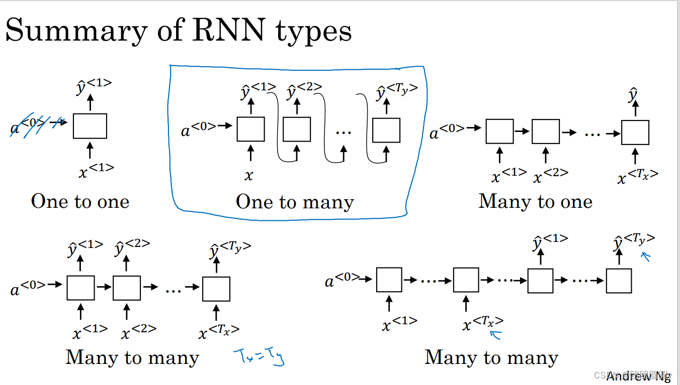
图3. 多种类型的RNN模型

1.2 解决RNN的梯度消失

和深度神经网络一样，RNN同样存在梯度消失和梯度爆炸的问题（复合函数求导，若每一步梯度>1则容易产生梯度爆炸，梯度<1则容易产生梯度消失，参见https://zhuanlan.zhihu.com/p/68579467），导致更新网络参数无效或者震荡太大。梯度爆炸容易观察，但是梯度消失不易观察，针对RNN，专门有GRU和LSML两种模型解决。

GRU简单理解为，每个时刻 $t$ 引入一个记忆值 $c^{t}$ ,记忆值 $c^{t}$ 和激活值 $a^{t}$ 相等。根据门控 $\Gamma _{u}$ （gate）决定是否用新得到的 $\tilde{c}^{<t>}$ 更新当前的c^{t},

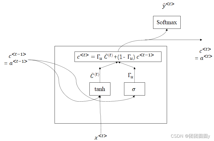
图4. GRU示意图

更新公式如下：

$\tilde{c}^{<t>} = tanh(W_{c}\begin{bmatrix} \Gamma_{r} c^{<t-1>} \\ x^{<t>} \end{bmatrix}+ b_{c})$ （2.1）

$\Gamma_{u} = tanh(W_{u}\begin{bmatrix} c^{<t-1>} \\ x^{<t>} \end{bmatrix}+ b_{u})$ （2.2）

$\Gamma_{r} = tanh(W_{r}\begin{bmatrix} c^{<t-1>} \\ x^{<t>} \end{bmatrix}+ b_{r})$ （2.3）

$c^{<t>} = \Gamma_{u} \tilde{c}^{<t>} + (1- \Gamma_{u})c^{<t-1>}$ （2.4）

$a^{<t>} = c^{<t>}$ （2.5）

与图4中只有一个门控 $\Gamma_{u}$ 不同的是，在计算 $\tilde{c}^{<t>}$ 的时候有另外一个相关性的门控 $\Gamma_r$ 。

LSMT和GRU不同的是， $a^{<t>}$ 和 $c^{<t>}$ 并不相等，引入了其他的门控 $\Gamma_{f}$ 和 $\Gamma_{o}$ ,其中 $\Gamma_{f}$ 取代了式（2.4）中的 $(1- \Gamma_{u})$ ，作为单独的遗忘门控； $\Gamma_{o}$ 用以更新激活值 $a^{<t>}$ ，如下：

$\tilde{c}^{<t>} = tanh(W_{c}\begin{bmatrix} c^{<t-1>} \\ x^{<t>} \end{bmatrix}+ b_{c})$ (3.1)

$\Gamma_{u} = tanh(W_{u}\begin{bmatrix} c^{<t-1>} \\ x^{<t>} \end{bmatrix}+ b_{u})$ (3.2)

$\Gamma_{f} = tanh(W_{f}\begin{bmatrix} c^{<t-1>} \\ x^{<t>} \end{bmatrix}+ b_{f})$ (3.3)

$\Gamma_{o} = tanh(W_{o}\begin{bmatrix} c^{<t-1>} \\ x^{<t>} \end{bmatrix}+ b_{o})$ (3.4)

$c^{<t>} = \Gamma_{u} \tilde{c}^{<t>} + \Gamma_{f}c^{<t-1>}$ (3.5)

$a^{<t>} = \Gamma_{o}c^{<t>}$ (3.6)

2. 实例

2.1 pytorch中语法

Torch.nn.RNN为内置的RNN网络。序列 $i$ 的激活值用 $h_{i}$ 表示，计算公式如下，

$h^{t} = tanh(W_{a}\begin{bmatrix} h^{t-1}\\ x^{t} \end{bmatrix} + b_{h})$

初始化一个RNN网络语法：

rnn=torch.nn.RNN(input_size, hidden_size, num_layers,nonlinearity, bias,batch_first,dropout, bidirectional)

参数

其中，一般用到的参数为input_size, hidden_size, num_layers,nonlinearity, bias,batch_first。

input_size：输入序列每个字节的维度
hidden_size：隐含层中的激活值的维度
num_layers：隐含层的层数

nonlinearity：默认：激活函数为tanh，也可以设置为relu等

bias：是否有偏重 $b_{h}$ ，默认为true

网络输入

Input—X：[seq_len, batch_size, input_size]
seq_len：输入的句子/序列的字节长度
batch_size：样本量
input_size：字节维度

Input—h0: [num_layers, batch_size, hidden_size]
num_layers：多少层隐含层，多少层的激活值
batch_size：样本量
hidden_size：激活值的维度

当网络的设置中batch_first为True时，输入为Input—X：[seq_len, batch_size, input_size]，Input—h0: [num_layers, batch_size, hidden_size]

网络输出

out-out（n-n类型RNN）
[seq_len,batch_size,hidden_size]
out-h（最后一个字节对应的激活值）
[seq_len,batch_size,hiden_size]

参加pytorch官网https://pytorch.org/docs/stable/generated/torch.nn.RNN.html#torch.nn.RNN、（超详细！！）Pytorch循环神经网络（RNN）快速入门与实战_Hello3q3q的博客-CSDN博客_rnn循环神经网络

示例

设计一个含有2层隐含层的RNN，输入输出示意图如下，

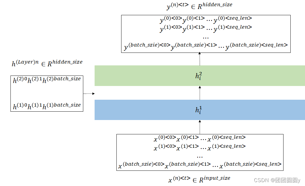
图5. 2层RNN输入批量数据输出示意图

在该例中，输入样本量 $batch_size = 2$ 的 $X$ ，序列长度 $seq_len = 3$ ，每个字节的维度为 $input_size = 10$ 。设计隐含层2层，激活值的维度为 $hidden_size = 3$ 。代码示例如下：


'''
RNN
input_size：输入序列每个字节的维度
hidden_size：隐含层中的激活值的维度
num_layers：隐含层的层数
Input—X
seq_len：输入的句子/序列的字节长度
batch_size：样本量
input_size：字节维度
Input—h(初始化的激活层)
num_layers：多少层隐含层，多少层的激活值
batch_size：样本量
hidden_size：激活值的维度
out-out
seq_len,batch_size,hidden_size
out-h
seq_len,batch_size,hiden_size
'''
input_size = 10
hidden_size = 3
num_layers = 2
output_size = 2
rnn = nn.RNN(input_size=input_size,hidden_size=hidden_size,
             num_layers=num_layers, batch_first=True)
 
seq_len = 3        
batch_size = 2      
x = torch.randn(batch_size,seq_len,input_size)        # 输入数据
h0 = torch.zeros(batch_size,num_layers,hidden_size)   # 输入数据
 
out, h = rnn(x, h0)  # 输出数据
linear = nn.Linear(hidden_size, output_size)
 
print("out.shape:",out.shape)
print("h.shape:",h.shape)
print("out",out)
out = linear(out)
print(out)

其中，linear层将输出 $out$ 由 $hidden\_size$ 的维度转变为我们想要的维度 $output\_size$ 。

结果如下，


out.shape: torch.Size([2, 3, 3])  # [batch_size, seq_len, hidden_size]
h.shape: torch.Size([2, 2, 3])    # [batch_size, Layers_num, hidden_size]
out tensor([[[-0.1594, -0.4284, -0.0468],    # 样本1字节1
         [ 0.0161, -0.5916, -0.1567],        # 样本1字节2
         [-0.0266, -0.6426, -0.1186]],       # 样本1字节3
 
        [[ 0.1776,  0.2767,  0.3266],        # 样本2字节1
         [ 0.0168,  0.1360,  0.0264],        # 样本2字节2
         [ 0.1708, -0.0948,  0.2696]]], grad_fn=<TransposeBackward1>)     # 样本2字节3
tensor([[[-0.2269, -0.0797],    # 样本1字节1
         [-0.1802,  0.0406],    # 样本1字节2
         [-0.1426,  0.0049]],   # 样本1字节1
 
        [[-0.7844, -0.0692],    # 样本2字节1
         [-0.6108, -0.0201],    # 样本2字节2
         [-0.5674, -0.0560]]], grad_fn=<AddBackward0>)    # 样本2字节1

（注：这里，为方便理解，RNN的参数batch_first=True，初始化x和h0的时候使用了对应的顺序，但是规范的方法应该是使用torch.nn.utils.rnn.PackedSequence）

2.2 网络训练

构建RNN模型，训练网络


class RNN_model(torch.nn.Module):
    def __init__(self, input_size, hidden_size,num_layers, output_size):
        super(RNN_model,self).__init__()
        self.rnn = nn.RNN(input_size = input_size,
                      hidden_size = hidden_size,
                      num_layers = num_layers,
                      batch_first=False)                     
        self.linear = nn.Linear(hidden_size, output_size)
    def forward(self, x, h0):
        out, h = self.rnn(x, h0)
        out = self.linear(out)
        return out
 
input_size = 10
hidden_size = 3
num_layers = 2
output_size = 2
model = RNN_model(input_size, hidden_size, num_layers, output_size)
model = model.to(device)

使用GRU训练，基本一致，将nn.RNN替换为nn.GRU


class RNN_model(torch.nn.Module):
    def __init__(self, input_size, hidden_size,num_layers, output_size):
        super(RNN_model,self).__init__()
        self.gru = nn.GRU(input_size = input_size,
                         hidden_size = hidden_size,
                         num_layers = num_layers,
                         batch_first=False)     
        self.linear = nn.Linear(hidden_size, output_size)
    def forward(self, x, h0):
        out, h = self.gru(x, h0)
        out = self.linear(out)
        return out
 
input_size = 10
hidden_size = 3
num_layers = 2
output_size = 2
model = RNN_model(input_size, hidden_size, num_layers, output_size)
model = model.to(device)

训练过程如下，


seq_len = 3        # 句子长度
batch_size = 2      
x = torch.randn(seq_len,batch_size,input_size)        # 输入数据
h0 = torch.zeros(num_layers,batch_size,hidden_size)   # 输入数据
target = torch.randn(seq_len,batch_size,output_size)  # 输出数据
 
board = SummaryWriter('/kaggle/working/ML_RNN/logs')
loss_function = nn.MSELoss()
opt = torch.optim.Adam(model.parameters(), lr=0.003, weight_decay=1e-3)
Epochs = 100
for epoch in range(Epochs):
    pred = model(x, h0)
    loss = loss_function(pred, target)
    #一般下面三行指令是放一起的
    opt.zero_grad()
    loss.backward()
    opt.step() 
    print('epoch=',epoch,' train_loss=',loss.item())
    board.add_scalar("Train_loss", loss.item(), epoch)
board.close()

误差图如下，

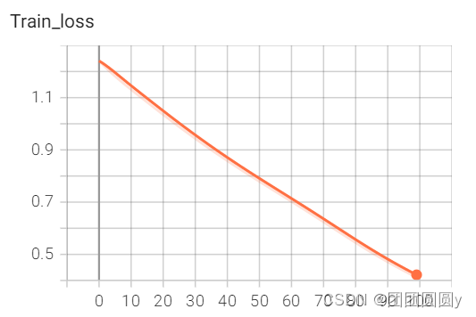
图6. 误差图

从误差图可以看到，训练到100步的时候，还未收敛。

本文内容由网友自发贡献，转载请注明出处：【wpsshop博客】