SVM兵王问题详解_clear all;fid = fopen('krkopt.data');c = fread(fid

（一） 识别系统的性能度量

1. 上接纸面笔记记录：
2. 不能仅用识别率来判断系统的性能。单纯用系统的识别率来判断系统的好坏，是没有意义的。例如，瞎猜的准确率为80%，那么你svm识别率为%95，那么还算高吗？

（1）几个重要的度量系统性能的标准

（1）混淆矩阵（confusion matrix）

1.0 解释上图：
TP: T 代表正确true, TP代表读正样本（positive）正确;对了，把P读成P
TN: T代表正确true, N，negative,TN 代表读负样本正确；对了，把N读成N
FP：代表读正样本错误；错了，读成P（把谁读成P会错呢？）
FN：代表读负样本错误；错了，读成N
显然，正负样本的总数是固定的；那么可以概率化，归一化；
2.0 那么系统的识别率是多少呢？
	识别成功个数：TP+TN; 总个数： TP+TN+FP+FN; 除一下就可以。99.61%
3.0 瞎猜的概率：由于负样本过多，所以全为负样本：TN + FP   89.96%
显然，这样的结果还可以，但是并不是非常好。
1
2
3
4
5
6
7
8
9
10

概率形式：

1.0 显然：TP+FN = 1;  FP+TN = 1;
2.0 见下图：
1
2

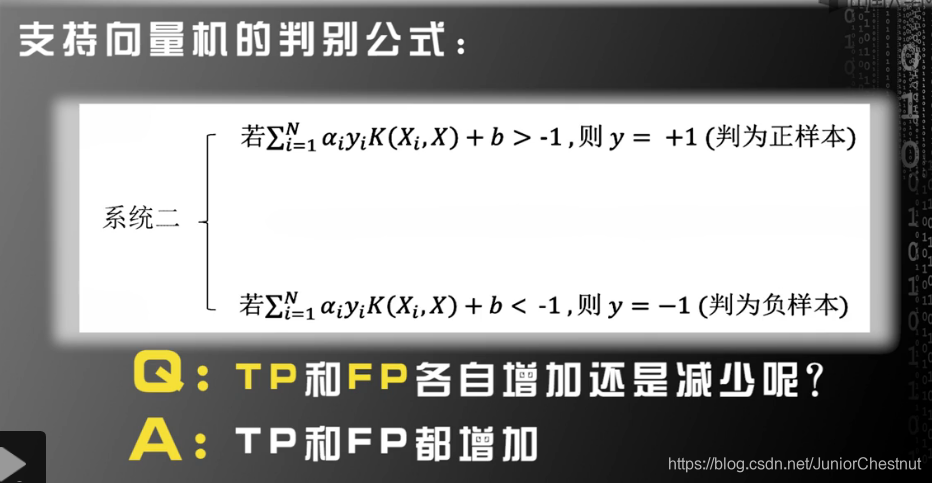
【注】因为阈值下降，TP和FP通过率都上去（为正的概率）

（2）引入ROC曲线

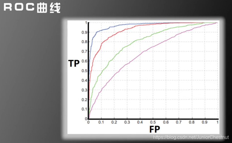
1.0 解释ROC曲线：是以FP和TP为横终坐标画成；
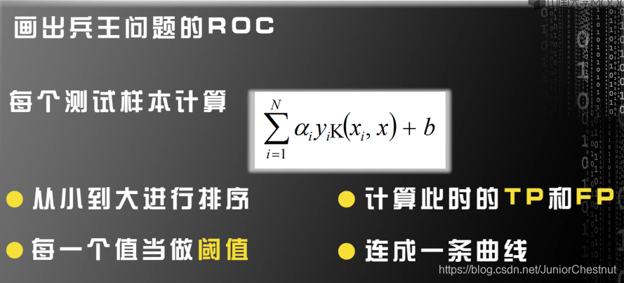
2.0 对每个测试样本，计算上图公式：
3.0 然后 将得到的值从小到大开始排序；
4.0 把每一个值当作阈值，计算此时的TP和FP；连成一条曲线；
1
2
3
4

（2.1）通过ROC曲线获得系统性能度量

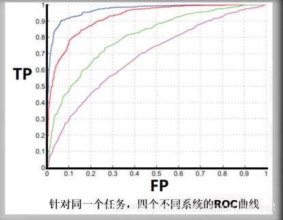
蓝色线最好，紫色线最差；因为在FP不变的情况下，TP越大越好。

（2.2）AUC指标

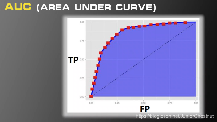
阴影面积越大越好。

（2.3）ERR

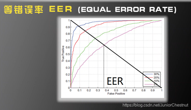
画一条45度线，EER为交点处的横坐标，显然，EER越小越好。

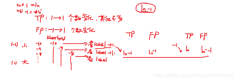
（2.4）ROC曲线代码解析

关键部分：通过当前得label去计算下一个得TP和FP

%Test the model on the remaining testing data and obtain the recognition rate.
clear all;
load model.mat;
load xTesting.mat;
load yTesting.mat;
% yPred 是对每个样本预测的标签； accuracy是在测试集上整体的识别率
% decisionValue: 是w^TX + b 的值；就是根据这个值贴标签
[yPred,accuracy,decisionValues] = svmpredict(yTesting,xTesting,model); 

%draw ROC                                  
[totalScores,index]  = sort(decisionValues);  % 先排序
labels = yTesting;
for i = 1:length(labels)
    labels(i) = yTesting(index(i)); % 将decisionValue与标签值对应起来。
end;


truePositive = zeros(1,length(totalScores)+1);
trueNegative = zeros(1,length(totalScores)+1);
falsePositive = zeros(1,length(totalScores)+1);
falseNegative = zeros(1,length(totalScores)+1);

% 计算TP和FP的总的个数. 索引数一直为1；
for i = 1:length(totalScores)
    if labels(i) == 1
        truePositive(1) = truePositive(1)+1; 
    else
        falsePositive(1) = falsePositive(1) +1;
    end;
end;

% FP: 是如何得出来的： 原本是不能通过，认成了pass, label = -1;
% 由于排好序列了，那么，TP 和 FP的个数，其实是递减的。
for i = 1:length(totalScores)
   if labels(i) == 1
       truePositive(i+1) = truePositive(i)-1;
       falsePositive(i+1) = falsePositive(i);
   else
       falsePositive(i+1) = falsePositive(i)-1;
       truePositive(i+1) = truePositive(i);
   end;
end;

% 概率化；
truePositive = truePositive/truePositive(1);
falsePositive = falsePositive/falsePositive(1);
plot(falsePositive, truePositive);

inc = 0.001;
startIndex = 1;
endIndex = length(falsePositive)
pointerIndex = 1;
pointerValue = falsePositive(1);
newFalsePositive = [];
newTruePositive = [];
while pointerIndex<=length(falsePositive)
    while pointerIndex<=length(falsePositive) && falsePositive(pointerIndex)>falsePositive(startIndex)-inc 
        pointerIndex = pointerIndex +1;
    end;
    newFalsePositive = [newFalsePositive, falsePositive(startIndex)];
    newTruePositive = [newTruePositive, mean(truePositive(startIndex:min(pointerIndex,length(truePositive))))];
    startIndex = pointerIndex;
end;
plot(newFalsePositive, newTruePositive);
1
2
3
4
5
6
7
8
9
10
11
12
13
14
15
16
17
18
19
20
21
22
23
24
25
26
27
28
29
30
31
32
33
34
35
36
37
38
39
40
41
42
43
44
45
46
47
48
49
50
51
52
53
54
55
56
57
58
59
60
61
62
63
64

clear all;
% Read the data.

fid  =  fopen('krkopt.DATA');
c = fread(fid, 3);

vec = zeros(6,1);
xapp = [];  % 接收六维的数据，先声明
yapp = [];  % 接收所有的标签，先声明

while ~feof(fid)
    string = [];
    c = fread(fid,1);
    flag = flag+1;
    while c~=13     % 13代表回车； // 这里是读一行
        string = [string, c];
        c=fread(fid,1);
    end;   
    fread(fid,1);                % 这里是处理一行               
    if length(string)>10
        vec(1) = string(1) - 96; % 把a变为整数1；
        vec(2) = string(3) - 48;
        vec(3) = string(5) - 96;
        vec(4) = string(7) - 48;
        vec(5) = string(9) - 96;
        vec(6) = string(11) - 48;
        xapp = [xapp,vec];
        if string(13) == 100  % 13是因为第13个是draw（和棋）100是d；
            yapp = [yapp,1];
        else
            yapp = [yapp,-1];
        end;
    end;
end;
fclose(fid);

[N,M] = size(xapp);  % [N,M]是获取xapp的维度，例如3*4，N = 3,M = 4
p = randperm(M);     % 直接打乱了训练样本，并且把列数作为行向量保存
                     % 1~M的整数随机置换
numberOfSamplesForTraining = 5000;
xTraining = [];
yTraining = [];
for i=1:numberOfSamplesForTraining
    xTraining  = [xTraining,xapp(:,p(i))]; % 这是从总样本中，取随机一列的全部元素
    yTraining = [yTraining,yapp(p(i))];    % 这是取上面元素对应的标签
end;
xTraining = xTraining'; % 取转置
yTraining = yTraining';

xTesting = [];
yTesting = [];
for i=numberOfSamplesForTraining+1:M       % 遍历剩下的数据作为测试数据
    xTesting  = [xTesting,xapp(:,p(i))];   % 注意同样用的p(i)
    yTesting = [yTesting,yapp(p(i))];
end;
xTesting = xTesting'; % 取转置
yTesting = yTesting';

%%%%%%%%%%%%%%%%%%%%%%%%
%Normalization 归一化
[numVec,numDim] = size(xTraining);
avgX = mean(xTraining);  % 这里是对每一列求平均值
stdX = std(xTraining);   % 对每一列求方差
for i = 1:numVec       % 以行遍历所有数据
    xTraining(i,:) = (xTraining(i,:)-avgX)./stdX;
end;
[numVec,numDim] = size(xTesting);

for i = 1:numVec
    xTesting(i,:) = (xTesting(i,:)-avgX)./stdX;
end;



%%%%%%%%%%%%%%%%%%%%%%%%%%%%%%%%%%
%SVM Gaussian kernel 
%Search for the optimal C and gamma, K(x1,x2) = exp{-||x1-x2||^2/gamma} to
%make the recognition rate maximum. 

%Firstly, search C and gamma in a crude scale (as recommended in 'A practical Guide to Support Vector Classification'))
CScale = [-5, -3, -1, 1, 3, 5,7,9,11,13,15];
gammaScale = [-15,-13,-11,-9,-7,-5,-3,-1,1,3];
C = 2.^CScale;
gamma = 2.^gammaScale;
maxRecognitionRate = 0;
for i = 1:length(C)  % 找到最佳的超参数 c 和 gama 的下标
    for j = 1:length(gamma)   % svm训练参数设置：
        cmd=['-t 2 -c ',num2str(C(i)),' -g ',num2str(gamma(j)),' -v 5'];
        recognitionRate = svmtrain(yTraining,xTraining,cmd); %训练数据和参数
        if recognitionRate>maxRecognitionRate
            maxRecognitionRate = recognitionRate
            maxCIndex = i;
            maxGammaIndex = j;
        end;
    end;
end;

%Then search for optimal C and gamma in a refined scale. 
n = 10; % 用最好的超参数，重新训练 %max 是返回最大的数
minCScale = 0.5*(CScale(max(1,maxCIndex-1))+CScale(maxCIndex));
maxCScale = 0.5*(CScale(min(length(CScale),maxCIndex+1))+CScale(maxCIndex));
newCScale = [minCScale:(maxCScale-minCScale)/n:maxCScale];

minGammaScale = 0.5*(gammaScale(max(1,maxGammaIndex-1))+gammaScale(maxGammaIndex));
maxGammaScale = 0.5*(gammaScale(min(length(gammaScale),maxGammaIndex+1))+gammaScale(maxGammaIndex));
newGammaScale = [minGammaScale:(maxGammaScale-minGammaScale)/n:maxGammaScale];
newC = 2.^newCScale;
newGamma = 2.^newGammaScale;
maxRecognitionRate = 0;
for i = 1:length(newC)
    for j = 1:length(newGamma)
        cmd=['-t 2 -c ',num2str(newC(i)),' -g ',num2str(newGamma(j)),' -v 5'];
        recognitionRate = svmtrain(yTraining,xTraining,cmd);
        if recognitionRate>maxRecognitionRate
            maxRecognitionRate = recognitionRate
            maxC = newC(i);
            maxGamma = newGamma(j);
        end;
    end;
end;

%Train the SVM model by the optimal C and gamma.
cmd=['-t 2 -c ',num2str(maxC),' -g ',num2str(maxGamma)];
model = svmtrain(yTraining,xTraining,cmd);
save model.mat model;
save xTesting.mat xTesting;
save yTesting.mat yTesting;

% plot(falsePositive,truePositive);




1
2
3
4
5
6
7
8
9
10
11
12
13
14
15
16
17
18
19
20
21
22
23
24
25
26
27
28
29
30
31
32
33
34
35
36
37
38
39
40
41
42
43
44
45
46
47
48
49
50
51
52
53
54
55
56
57
58
59
60
61
62
63
64
65
66
67
68
69
70
71
72
73
74
75
76
77
78
79
80
81
82
83
84
85
86
87
88
89
90
91
92
93
94
95
96
97
98
99
100
101
102
103
104
105
106
107
108
109
110
111
112
113
114
115
116
117
118
119
120
121
122
123
124
125
126
127
128
129
130
131
132
133