
img = cv.imread("car.jpg")
 
#获取三个通道的数值
px = img[100, 100]
print(px)
#只获取蓝色通道的数值,绿色-1，红色-2
blue = img[100, 100, 0]
print(blue)
#修改一点的像素值
img[100, 100] = [255, 255, 255]
print(img[100, 100])
 
#官方说用下面的方法进行像素值获取和进行修改更好,但是只有返回scalar--标量，所以只能单个通道选择
red = img.item(100, 100, 2)
print(red)
 
img.itemset((100, 100, 2),100)
red2 = img.item(100, 100, 2)
print(red2)

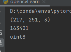
②、获取图像的特性


img = cv.imread("car.jpg")
 
print(img.shape)  #如果是灰度图，那么就只有两个坐标参数
print(img.size)
print(img.dtype) #dtype = datatype,数据类型容易导致错误

③、ROI regions of images, 图像的感兴趣区域

文档里，梅西提的足球是感兴趣区域，并在图中的另一处区域进行了复制

④、分离和融合图像通道


img = cv.imread("test1.jpg")
 
#三个通道的分离和融合
b, g, r = cv.split(img)
img1 = cv.merge((b, g, r))
 
#只需要分离一个通道
b = img[:,:,0] #blue - 0
#使得某个通道的像素全为某个值
img[:,:,2] = 0  #红色像素全部为零

如非必要，不用使用cv.split分离通道，耗时大，一般用numpy的索引即可

⑤、为图片创建一边界 use cv.copyMakeBorder()


import cv2 as cv
import numpy as np
from matplotlib import pyplot as plt
 
BLUE = [255 ,0 ,0]
 
img1 = cv.imread('car.jpg')
 
replicate = cv.copyMakeBorder(img1 ,10 ,10 ,10 ,10 ,cv.BORDER_REPLICATE)
reflect = cv.copyMakeBorder(img1 ,10 ,10 ,10 ,10 ,cv.BORDER_REFLECT)
reflect101 = cv.copyMakeBorder(img1 ,10 ,10 ,10 ,10 ,cv.BORDER_REFLECT_101)
wrap = cv.copyMakeBorder(img1 ,10 ,10 ,10 ,10 ,cv.BORDER_WRAP)
constant= cv.copyMakeBorder(img1 ,10 ,10 ,10 ,10 ,cv.BORDER_CONSTANT ,value=BLUE)
 
plt.subplot(231) ,plt.imshow(img1 ,'gray') ,plt.title('ORIGINAL')
plt.subplot(232) ,plt.imshow(replicate ,'gray') ,plt.title('REPLICATE')
plt.subplot(233) ,plt.imshow(reflect ,'gray') ,plt.title('REFLECT')
plt.subplot(234) ,plt.imshow(reflect101 ,'gray') ,plt.title('REFLECT_101')
plt.subplot(235) ,plt.imshow(wrap ,'gray') ,plt.title('WRAP')
plt.subplot(236) ,plt.imshow(constant ,'gray') ,plt.title('CONSTANT')
 
plt.show()

下面的话解释了为什么蓝色变成了红色，整体的颜色都发生了反相

2、图片的数学操作

①、加法，其中opencv的add函数是饱和运算，numpy 的加法是模运算

以图片形式进行融合的代码如下，这里将两张图片的shape进行匹配后才能相加


img1 = cv.imread('car.jpg')
print(img1.shape)
print(img1.size)
print(img1.dtype)
img1 = cv.resize(img1,(1600,900))
print(img1.shape)
print(img1.size)
print(img1.dtype)
 
print("jijsijai")
 
img2 = cv.imread('test1.jpg')
print(img2.shape)
print(img2.size)
print(img2.dtype)
 
img3 = cv.add(img1,img2)
 
cv.imshow('test',img3)
# 等待任意输入
cv.waitKey(0)
cv.destroyAllWindows();

②、图像融合操作，将两张图片按照一定权重相加

③、位运算


back = cv.imread('dota1.jpg')
logo = cv.imread('dota2.jpg')
 
# 目标把图标放到右下角，所以创建ROI
row1, col1, channel1 = back.shape #背景的大小
row2, col2, channel2 = logo.shape #logo的大小
roi = back[row1-row2:row1, col1 - col2:col1]
 
# Now create a mask of logo and create its inverse mask also
logogray = cv.cvtColor(logo,cv.COLOR_BGR2GRAY)
ret, mask = cv.threshold(logogray, 10, 255, cv.THRESH_BINARY) #设定阈值对logo中的像素进行过滤
mask_inv = cv.bitwise_not(mask) #取反操作
 
# Now black-out the area of logo in ROI
img1_bg = cv.bitwise_and(roi,roi,mask = mask_inv)  #使得感兴趣区域像素全为0
 
# Take only region of logo from logo image.
img2_fg = cv.bitwise_and(logo,logo,mask = mask)
 
# Put logo in ROI and modify the main image
dst = cv.add(img1_bg, img2_fg)
back[row1-row2:row1, col1 - col2:col1] = dst
 
cv.imshow('res', back)
cv.waitKey(0)
cv.destroyAllWindows()

3、代码性能检测与提升手段

①、Measuring Performance with OpenCV

在代码的首尾减一下，计算可得程序的运行时间，以s为单位

上一段的代码的执行时间0.31s

用python 自带的time.time得到

②、一些代码优化的技巧

1--减少循环操作

2--尽量向量化算法

3--缓存一致性，：）？？？？，不是我这种fw考虑的吧

4-- 减少数组（序列）的复制操作

二、图像处理的方法

1、改变图像的颜色空间

①、常用的颜色空间

图像空间中经常用到的就三个BGR、GRAY、HSV

注意HSV 的范围

②、hsv中的物体提取

在hsv 颜色空间中更加容易用颜色特征提取出一个物体

官方的代码，对视频中的蓝色物体进行追踪


import cv2 as cv
import numpy as np
 
cap = cv.VideoCapture(0)
 
while(1):
 
    # Take each frame
    _, frame = cap.read()
 
    # Convert BGR to HSV
    hsv = cv.cvtColor(frame, cv.COLOR_BGR2HSV)
 
    # define range of blue color in HSV
    lower_blue = np.array([110,100,100])
    upper_blue = np.array([130,255,255])
 
    # Threshold the HSV image to get only blue colors
    mask = cv.inRange(hsv, lower_blue, upper_blue)
 
    # Bitwise-AND mask and original image
    res = cv.bitwise_and(frame,frame, mask= mask)
 
    cv.imshow('frame',frame)
    cv.imshow('mask',mask)
    cv.imshow('res',res)
    k = cv.waitKey(5) & 0xFF
    if k == 27:
        break
 
cv.destroyAllWindows()

③、如何找HSV值进行跟踪

官方给了一种通用方法

计算之前的蓝色追踪的hsv


#以上一个找蓝色的代码为例
blue = np.uint8([[[255, 0, 0 ]]])
hsv_blue = cv.cvtColor(blue,cv.COLOR_BGR2HSV)
print(hsv_blue)

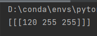
120-10 = 110; 120+10 = 130 符合预期

2、图像的几何变换

①、尺寸修改

②、图片位置的移动

使用cv.warpAffine()，其中变换矩阵

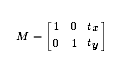
注意，row对应高度，col对应宽度


img = cv.imread('car.jpg', 0)
rows, cols = img.shape
 
M = np.float32([[1, 0, 100], [0, 1, 50]])
dst = cv.warpAffine(img, M, (cols, rows))
 
cv.imshow('img', dst)
cv.waitKey(0)
cv.destroyAllWindows()

③、图片旋转一定角度

opencv 提供一种可以在图片中心按照一个角度进行旋转


img = cv.imread('car.jpg', 0)
rows, cols = img.shape
 
# cols-1 and rows-1 are the coordinate limits.对应的是参数是图片的中心
M = cv.getRotationMatrix2D(((cols-1)/2.0,(rows-1)/2.0),90,1)
dst = cv.warpAffine(img,M,(cols,rows))
 
cv.imshow('img', dst)
cv.waitKey(0)
cv.destroyAllWindows()

④、仿射变换

在仿射变换中，变换后之前的线依然保持平行。设输入图像的三个点，输出图像的三个点，使用 cv.getAffineTransform 求出变换矩阵

官方的实例

⑤、视角变换

注意点，找的四个点中至少三个不在一条线上，效果，原图的四个顶点由选择的四个点进行顶替

3、图像阈值处理

①、简单阈值化，二值化处理

阈值处理简单说就是，一个像素其值小于阈值设为0，大于阈值设为最大值

cv.threshold。函数返回的第一个数是阈值，第二个数是阈值处理后的函数

一般阈值化前先要转为灰度图像


import cv2 as cv
import numpy as np
from matplotlib import pyplot as plt
 
from matplotlib import pyplot as plt
 
img = cv.imread('bw.jpg', 0)
ret, thresh1 = cv.threshold(img, 127, 255, cv.THRESH_BINARY)
ret, thresh2 = cv.threshold(img, 127, 255, cv.THRESH_BINARY_INV)
ret, thresh3 = cv.threshold(img, 127, 255, cv.THRESH_TRUNC)
ret, thresh4 = cv.threshold(img, 127, 255, cv.THRESH_TOZERO)
ret, thresh5 = cv.threshold(img, 127, 255, cv.THRESH_TOZERO_INV)
 
titles = ['Original Image', 'BINARY', 'BINARY_INV', 'TRUNC', 'TOZERO', 'TOZERO_INV']
images = [img, thresh1, thresh2, thresh3, thresh4, thresh5]
 
for i in range(6):
    plt.subplot(2, 3, i + 1), plt.imshow(images[i], 'gray', vmin=0, vmax=255)
    plt.title(titles[i])
    plt.xticks([]), plt.yticks([])
 
plt.show()

②、适应性阈值化

适应性阈值化针对多种光源的情况，这个算法决定一个像素点阈值时是根据周围一小部分区域，所以我们在图像的不同区域得到不同阈值，不同区域用不同的阈值进行处理


import cv2 as cv
import numpy as np
from matplotlib import pyplot as plt
 
img = cv.imread('car.jpg', 0)
img = cv.medianBlur(img, 5)
 
ret, th1 = cv.threshold(img, 127, 255, cv.THRESH_BINARY)
th2 = cv.adaptiveThreshold(img, 255, cv.ADAPTIVE_THRESH_MEAN_C, \
                           cv.THRESH_BINARY, 11, 2)
th3 = cv.adaptiveThreshold(img, 255, cv.ADAPTIVE_THRESH_GAUSSIAN_C, \
                           cv.THRESH_BINARY, 11, 2)
 
titles = ['Original Image', 'Global Thresholding (v = 127)',
          'Adaptive Mean Thresholding', 'Adaptive Gaussian Thresholding']
images = [img, th1, th2, th3]
 
for i in range(4):
    plt.subplot(2, 2, i + 1), plt.imshow(images[i], 'gray')
    plt.title(titles[i])
    plt.xticks([]), plt.yticks([])
plt.show()

③、Otsu's Binarization 大津二值化算法

Otsu's method avoids having to choose a value and determines it automatically.这个算法不需要自己设定阈值

Similarly, Otsu's method determines an optimal global threshold value from the image histogram.

是因为这个算法可以从灰度直方图中自己确定阈值

官方的例子如下，三种方法进行比较，明显第三个方法，先滤波去噪声，在ostu二值化

4、图像平滑处理 Smoothing Images

①、二维卷积滤波

卷积， The operation works like this: keep this kernel above a pixel, add all the 25 pixels below this kernel, take the average, and replace the central pixel with the new average value.

官方的核函数以平均滤波为例


import cv2 as cv
import numpy as np
from matplotlib import pyplot as plt
 
img1 = cv.imread('dota2.jpg')
 
 
kernal = np.ones((5,5),np.float32)/25
img2 = cv.filter2D(img1,-1,kernal)
 
images = [img1,img2]
titles = ['Original Image', 'dst Image']
 
for i in range(2):
    plt.subplot(1,2,i+1),plt.imshow(images[i],'gray')
    plt.title(titles[i])
    plt.xticks([]), plt.yticks([])
 
plt.show()

②、图像模糊即图像平滑

Image blurring is achieved by convolving the image with a low-pass filter kernel. It is useful for removing noise. It actually removes high frequency content (eg: noise, edges) from the image. So edges are blurred a little bit in this operation (there are also blurring techniques which don't blur the edges). OpenCV provides four main types of blurring techniques.

图像平滑处理的实现就是基于上面的图像的二维卷积，低通滤波处理，除去噪声、边缘，所以会造成模糊的结果。opencv 提供四种模糊的方法

第一种、Averaging，使用cv.blur函数

第二种、Gaussian Blurring，Gaussian blurring is highly effective in removing Gaussian noise from an image，去除高斯噪声很有用

第三种、Median Blurring，This is highly effective against salt-and-pepper noise in an image.椒盐噪声

第四种、Bilateral Filtering，cv.bilateralFilter() is highly effective in noise removal while keeping edges sharp. 去除噪声时保持边缘的区分度


import cv2 as cv
import numpy as np
from matplotlib import pyplot as plt
 
img1 = cv.imread('car.jpg',0)
 
 
img2 = cv.blur(img1,(5,5))
img3 = cv.GaussianBlur(img1,(5,5),0)
img4 = cv.medianBlur(img1,5)
img5= cv.bilateralFilter(img1,9,75,75)
 
images = [img1,img2,img3,img4,img5]
titles = ['Original Image', 'Average Blur Image', 'Gaussing Blur Img', 'Media Blur Img',' Bilateral Filtering']
 
for i in range(5):
    plt.subplot(2,3,i+1),plt.imshow(images[i],'gray')
    plt.title(titles[i])
    plt.xticks([]), plt.yticks([])
 
plt.show()

5、形态学处理 Morphological Transformations

①、腐蚀、Erosion

it erodes away the boundaries of foreground object (Always try to keep foreground in white)

腐蚀的是前景对象，一般在二值化图像中，白色是前景对象

It is useful for removing small white noises (as we have seen in colorspace chapter), detach two connected objects etc.

可以用于不同对象之间的分离

腐蚀的原理， A pixel in the original image (either 1 or 0) will be considered 1 only if all the pixels under the kernel is 1, otherwise it is eroded (made to zero).

②、膨胀 Dilation

It is just opposite of erosion.


import cv2 as cv
import numpy as np
from matplotlib import pyplot as plt
 
img = cv.imread('6.jpg',0)
 
img = cv.resize(img,(100,200))
ret, imgT = cv.threshold(img,100,255,cv.THRESH_BINARY)
 
kernel = np.ones((5,5),np.uint8)
imgE = cv.erode(imgT,kernel,iterations = 1) #iterations , 迭代
imgD = cv.dilate(imgT,kernel,iterations = 1)
 
images = [imgT, imgE, imgD]
titles = ['Original Image', 'Erode Image', 'Dilation Image']
 
for i in range(3):
    plt.subplot(1,3,i+1),plt.imshow(images[i],'gray')
    plt.title(titles[i])
    plt.xticks([]), plt.yticks([])
 
plt.show()

③、开运算、闭运算

开运算 Opening

erosion followed by dilation，先腐蚀后膨胀

It is useful in removing noise, as we explained above.

闭运算 Closing

Dilation followed by Erosion.，先膨胀后腐蚀

It is useful in closing small holes inside the foreground objects, or small black points on the object.就是将前景图像（白色图像）里的小黑点给闭合了

④、梯度处理 Morphological Gradient

The result will look like the outline of the object.保留前景图像的轮廓


import cv2 as cv
import numpy as np
from matplotlib import pyplot as plt
 
img = cv.imread('6.jpg',0)
 
img = cv.resize(img,(100,200))
ret, imgT = cv.threshold(img,100,255,cv.THRESH_BINARY)
 
kernel = np.ones((5,5),np.uint8)
gradient = cv.morphologyEx(img, cv.MORPH_GRADIENT, kernel)
 
cv.imshow('test',gradient)
cv.waitKey(0)
cv.destroyAllWindows()

⑤、Top Hat and Black Hat

top-hat and black-hat transform are operations that are used to extract small elements and details from given images.

the top-hat transform is defined as the difference between the input image and its opening by some structuring element, while the black-hat transform is defined as the difference between the closing and the input image.

tophat 提取small elements


# Importing OpenCV
import cv2
 
 
# Getting the kernel to be used in Top-Hat
filterSize =(3, 3)
kernel = cv2.getStructuringElement(cv2.MORPH_RECT,
								filterSize)
 
# Reading the image named 'input.jpg'
input_image = cv2.imread("tophat.png")
input_image = cv2.cvtColor(input_image, cv2.COLOR_BGR2GRAY)
 
# Applying the Top-Hat operation
tophat_img = cv2.morphologyEx(input_image,
							cv2.MORPH_TOPHAT,
							kernel)
 
cv2.imshow("original", input_image)
cv2.imshow("tophat", tophat_img)
cv2.waitKey(5000)

blackhat 提取details


# Importing OpenCV and numpy
import cv2
 
# Defining the kernel to be used in Top-Hat
filterSize =(3, 3)
kernel = cv2.getStructuringElement(cv2.MORPH_RECT,
								filterSize)
 
# Reading the image named 'input.jpg'
input_image = cv2.imread("blackhat.jpg")
input_image = cv2.cvtColor(input_image, cv2.COLOR_BGR2GRAY)
 
# Applying the Black-Hat operation
tophat_img = cv2.morphologyEx(input_image,
							cv2.MORPH_BLACKHAT,
							kernel)
 
cv2.imshow("original", input_image)
cv2.imshow("tophat", tophat_img)
cv2.waitKey(5000)

⑥、结构化元素Structuring Element

But in some cases, you may need elliptical/circular shaped kernels. So for this purpose, OpenCV has a function, cv.getStructuringElement(). You just pass the shape and size of the kernel, you get the desired kernel.

官方文档的例子，矩形，椭圆，十字形的

6、图像的梯度处理（高通滤波）

OpenCV provides three types of gradient filters or High-pass filters, Sobel, Scharr and Laplacian.

注意

If you want to detect both edges, better option is to keep the output datatype to some higher forms, like cv.CV_16S, cv.CV_64F etc,

用sobel检测时要选用cv.CV_64F，这样才可以检测出两个内容

官方例子

7、Canny Edge Detection 边缘检测

Canny Edge Detection is a popular edge detection algorithm.

这个算法是多个步骤的合成，具体原理之后将，

效果


import numpy as np
import cv2 as cv
from matplotlib import pyplot as plt
 
img = cv.imread('car.jpg', 0)
edges = cv.Canny(img, 100, 200)
 
plt.subplot(121), plt.imshow(img, cmap='gray')
plt.title('Original Image'), plt.xticks([]), plt.yticks([])
plt.subplot(122), plt.imshow(edges, cmap='gray')
plt.title('Edge Image'), plt.xticks([]), plt.yticks([])
 
plt.show()

8、Image Pyramids 图像金字塔

These set of images with different resolutions are called Image Pyramids (because when they are kept in a stack with the highest resolution image at the bottom and the lowest resolution image at top, it looks like a pyramid).

图像金字塔是其他操作的基础原理

One application of Pyramids is Image Blending.其中一个应用就是图像的融合

官方


import numpy as np
import cv2 as cv
from matplotlib import pyplot as plt
 
 
A = cv.imread('apple.jpg')
A = cv.resize(A, (256, 256))
 
B = cv.imread('orange.jpg')
B = cv.resize(B, (256, 256))
 
# generate Gaussian pyramid for A
G = A.copy()
gpA = [G]
for i in range(6):
    G = cv.pyrDown(G)
    gpA.append(G)
#有点问题还没改
# generate Gaussian pyramid for B
G = B.copy()
gpB = [G]
for i in range(6):
    G = cv.pyrDown(G)
    gpB.append(G)
 
# generate Laplacian Pyramid for A
lpA = [gpA[5]]
for i in range(5, 0, -1):
    GE = cv.pyrUp(gpA[i])
    L = cv.subtract(gpA[i - 1], GE)
    lpA.append(L)
 
# generate Laplacian Pyramid for B
lpB = [gpB[5]]
for i in range(5, 0, -1):
    GE = cv.pyrUp(gpB[i])
    L = cv.subtract(gpB[i - 1], GE)
    lpB.append(L)
 
# Now add left and right halves of images in each level
LS = []
for la, lb in zip(lpA, lpB):
    rows, cols, dpt = la.shape
    ls = np.hstack((la[:, 0:cols // 2], lb[:, cols // 2:]))
    LS.append(ls)
 
# now reconstruct
ls_ = LS[0]
for i in range(1, 6):
    ls_ = cv.pyrUp(ls_)
    ls_ = cv.add(ls_, LS[i])
 
# image with direct connecting each half
real = np.hstack((A[:, :cols // 2], B[:, cols // 2:]))
 
 
images = [ls,real]
titles = ["Pyramid_blending","Direct_blending"]
 
for i in range(2):
    plt.subplot(2,1,i+1),plt.imshow(images[i],'gray')
    plt.title(titles[i])
    plt.xticks([]), plt.yticks([])
 
plt.show()

我的例子，奇怪了，：《

9、对图像轮廓的操作 Contours

①、简介

Contours is a Python list of all the contours in the image. Each individual contour is a Numpy array of (x,y) coordinates of boundary points of the object. 返回的轮廓使一个序列，保存着找到的所有轮廓

画轮廓的方法

②、轮廓特征，将轮廓在原图中进行标识

图像矩，Image moments ，From this moments, you can extract useful data like area, centroid etc.


import numpy as np
import cv2 as cv
 
img = cv.imread('bw.jpg', 0)
ret, thresh = cv.threshold(img, 127, 255, 0)
contours, hierarchy = cv.findContours(thresh, 1, 2)
 
cnt = contours[0]
M = cv.moments(cnt)
print(M)
 
cx = int(M['m10']/M['m00'])
cy = int(M['m01']/M['m00'])
 
area = cv.contourArea(cnt)
perimeter = cv.arcLength(cnt,True)
 
print("Centroid : ",cx,cy)
print("Contour Area : ", area)
print("perimeter : ",perimeter)

Contour Approximation，轮廓近似，修改参数大小改变得到的轮廓的近似程度


import numpy as np
import cv2 as cv
 
img = cv.imread('rect.png', 0)
ret, thresh = cv.threshold(img, 127, 255, 0)
contours, hierarchy = cv.findContours(thresh, 1, 2)
 
cnt = contours[0]
 
epsilon = 0.01*cv.arcLength(cnt,True)
approx1 = cv.approxPolyDP(cnt,epsilon,True)
 
epsilon = 0.001*cv.arcLength(cnt,True)
approx2 = cv.approxPolyDP(cnt,epsilon,True)
 
# 3.画出多边形
image = cv.cvtColor(img, cv.COLOR_GRAY2BGR)
cv.polylines(image, [approx1], True, (255, 0, 0), 2)
cv.polylines(image, [approx2], True, (0, 255, 0), 2)
 
print(len(approx1))  # 角点的个数
cv.imshow('approxPloyDP', image)
cv.waitKey(0)
cv.destroyAllWindows()

Convex Hull,凸包，与上面的轮廓近似的功能类似,找出图像中凸出来的点


import numpy as np
import cv2 as cv
 
img = cv.imread('hand.jpg', 0)
ret, thresh = cv.threshold(img, 235, 255, 0)
 
cv.imshow('thresh', thresh)
contours, hierarchy = cv.findContours(thresh, 2, 1)
 
print(len(contours))
 
 
 
# 寻找物体的凸包并绘制凸包的轮廓
for cnt in contours:
    hull = cv.convexHull(cnt)
    length = len(hull)
    # 如果凸包点集中的点个数大于5
    if length > 5:
        # 绘制图像凸包的轮廓
        for i in range(length):
            cv.line(img, tuple(hull[i][0]), tuple(hull[(i+1)%length][0]), (0,0,255), 2)
 
 
cv.imshow('test', img)
cv.waitKey(0)
cv.destroyAllWindows()

Bounding Rectangle，边界矩形，将轮廓用矩形给框出来，


import numpy as np
import cv2 as cv
 
img = cv.imread('hand.jpg',0)
ret, thresh = cv.threshold(img, 235, 255, 0)
contours, hierarchy = cv.findContours(thresh, 2, 1)
 
for cnt in contours:
    if len(cnt) > 100:
        x, y, w, h = cv.boundingRect(cnt)
        cv.rectangle(img, (x, y), (x + w, y + h), (0, 255, 0), 2)
 
 
cv.imshow('test',img)
 
cv.waitKey(0)
cv.destroyAllWindows()

Rotated Rectangle


import numpy as np
import cv2 as cv
 
img = cv.imread('hand.jpg',0)
ret, thresh = cv.threshold(img, 235, 255, 0)
contours, hierarchy = cv.findContours(thresh, 2, 1)
 
for cnt in contours:
    if len(cnt) > 100:
        rect = cv.minAreaRect(cnt)
        box = cv.boxPoints(rect)
        box = np.int0(box)
        cv.drawContours(img, [box], 0, (0, 0, 255), 2)
 
 
cv.imshow('test',img)
 
cv.waitKey(0)
cv.destroyAllWindows()

Minimum Enclosing Circle


import numpy as np
import cv2 as cv
 
img = cv.imread('hand.jpg',0)
ret, thresh = cv.threshold(img, 235, 255, 0)
contours, hierarchy = cv.findContours(thresh, 2, 1)
 
image  = cv.imread('hand.jpg')
for cnt in contours:
    if len(cnt) > 100:
        (x, y), radius = cv.minEnclosingCircle(cnt)
        center = (int(x), int(y))
        radius = int(radius)
        cv.circle(image, center, radius, (0, 255, 0), 2)
 
 
cv.imshow('test',image)
 
 
cv.waitKey(0)
cv.destroyAllWindows()

Fitting an Ellipse


import numpy as np
import cv2 as cv
 
img = cv.imread('hand.jpg',0)
ret, thresh = cv.threshold(img, 235, 255, 0)
contours, hierarchy = cv.findContours(thresh, 2, 1)
 
image  = cv.imread('hand.jpg')
for cnt in contours:
    if len(cnt) > 100:
        ellipse = cv.fitEllipse(cnt)
        cv.ellipse(image , ellipse, (0, 255, 0), 2)
 
 
cv.imshow('test',image)
 
 
cv.waitKey(0)
cv.destroyAllWindows()

③、Contour Properties 轮廓属性

Here we will learn to extract some frequently used properties of objects like Solidity, Equivalent Diameter, Mask image, Mean Intensity etc.

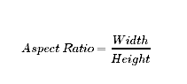
1. Aspect Ratio

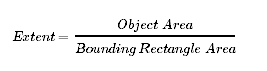
2.Extent

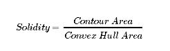
3.Solidity

4、Equivalent Diameter

5、Orientation

Orientation is the angle at which object is directed.

6、Mask

mask = np.zeros(imgray.shape,np.uint8)

常常在其它函数的调用中作为参数

Pixel Points

Maximum Value, Minimum Value and their locations

Mean Color or Mean Intensity


import numpy as np
import cv2 as cv
 
img = cv.imread('hand.jpg',0)
ret, thresh = cv.threshold(img, 235, 255, 0)
contours, hierarchy = cv.findContours(thresh, 2, 1)
 
#举例
cnt = contours[0]
x,y,w,h = cv.boundingRect(cnt)
aspect_ratio = float(w)/h
print('aspect_ratio = ',aspect_ratio)
 
area = cv.contourArea(cnt)
x,y,w,h = cv.boundingRect(cnt)
rect_area = w*h
extent = float(area)/rect_area
print('extent = ',extent)
 
area = cv.contourArea(cnt)
hull = cv.convexHull(cnt)
hull_area = cv.contourArea(hull)
solidity = float(area)/hull_area
print('solidity = ',solidity)
 
area = cv.contourArea(cnt)
equi_diameter = np.sqrt(4*area/np.pi)
print('equi_diameter  = ',equi_diameter)
 
(x,y),(MA,ma),angle = cv.fitEllipse(cnt)
print('orientation  = ',angle)
 
 
mask = np.zeros(img.shape,np.uint8)
pixelpoints = cv.findNonZero(mask)
print('pixelpoints',pixelpoints)
 
min_val, max_val, min_loc, max_loc = cv.minMaxLoc(img,mask = mask)
print('min_val, max_val, min_loc, max_loc =',min_val, max_val, min_loc, max_loc)
 
mean_val = cv.mean(img,mask = mask)
print('mean_val',mean_val)

7、Extreme Points

④、Contours : More Functions，更多功能

Convexity Defects，缺陷，以下图为例，标出来的轮廓与实际的轮廓的偏差就是defect


import cv2 as cv
import numpy as np
 
img = cv.imread('star.jpg')
img_gray = cv.cvtColor(img, cv.COLOR_BGR2GRAY)
ret, thresh = cv.threshold(img_gray, 127, 255, 0)
contours, hierarchy = cv.findContours(thresh, 2, 1)
cnt = contours[0]
 
hull = cv.convexHull(cnt, returnPoints=False)
defects = cv.convexityDefects(cnt, hull)
 
for i in range(defects.shape[0]):
    s, e, f, d = defects[i, 0]
    start = tuple(cnt[s][0])
    end = tuple(cnt[e][0])
    far = tuple(cnt[f][0])
    cv.line(img, start, end, [0, 255, 0], 2)
    cv.circle(img, far, 5, [0, 0, 255], -1)
 
cv.imshow('img', img)
cv.waitKey(0)
cv.destroyAllWindows()

Point Polygon Test

This function finds the shortest distance between a point in the image and a contour.

返回图像中一个点和一个轮廓的最短距离


import cv2 as cv
import numpy as np
 
img = cv.imread('star.jpg')
img_gray = cv.cvtColor(img, cv.COLOR_BGR2GRAY)
ret, thresh = cv.threshold(img_gray, 127, 255, 0)
contours, hierarchy = cv.findContours(thresh, 2, 1)
print(len(contours))
 
cnt = contours[0]
 
 
dist = cv.pointPolygonTest(cnt,(50,50),True)
 
print('the shortest distance', dist)

Match Shapes，比较两个图像的轮廓，返回一个度量值，越小，两张图像的相似度越高


import cv2 as cv
import numpy as np
 
img = cv.imread('star.jpg')
img2 = cv.imread('star2.png')
 
cv.imshow('star',img)
cv.imshow('star2',img2)
 
img_gray = cv.cvtColor(img, cv.COLOR_BGR2GRAY)
ret, thresh = cv.threshold(img_gray, 127, 255, 0)
contours, hierarchy = cv.findContours(thresh, 2, 1)
cnt = contours[0]
 
img2_gray = cv.cvtColor(img2,cv.COLOR_BGR2GRAY)
ret, thresh2 = cv.threshold(img2_gray, 127, 255, 0)
contours2, hierarchy = cv.findContours(thresh2, 2, 1)
cnt2 = contours2[0]
 
ret = cv.matchShapes(cnt,cnt2,1,0.0)
print('star and star2 simility',ret)
 
ret = cv.matchShapes(cnt,cnt,1,0.0)
print('star and star2 simility',ret)
 
cv.waitKey(0)
cv.destroyAllWindows()

Contours Hierarchy 轮廓的层次

What is Hierarchy?

In some cases, some shapes are inside other shapes. we call outer one as parent and inner one as child. This way, contours in an image has some relationship to each other.Representation of this relationship is called the Hierarchy.

10、灰度直方图 Histograms in OpenCV

①、 Find, Plot, Analyze !!!

Theory

histogram，which gives you an overall idea about the intensity distribution of an image.

图像的强度分布

X 轴，像素值分布；

Y轴，该像素值对应的像素数

！！！ Remember, this histogram is drawn for grayscale image, not color image

some terminologies related with histograms：

Bins:This each sub-part is called "BIN". In first case, number of bins were 256 (one for each pixel) while in second case, it is only 16. BINS is represented by the term histSize in OpenCV docs.就是x轴上有几个值

DIMS : It is the number of parameters for which we collect the data. In this case, we collect data regarding only one thing, intensity value. So here it is 1.

RANGE : It is the range of intensity values you want to measure. Normally, it is [0,256], ie all intensity values.

Find

Histogram Calculation in OpenCV

Histogram Calculation in Numpy

Plot

Using Matplotlib


import numpy as np
import cv2 as cv
from matplotlib import pyplot as plt
 
 
img = cv.imread('dota1.jpg')
 
color = ('b','g','r')
for i,col in enumerate(color):
    histr = cv.calcHist([img],[i],None,[256],[0,256])
    plt.plot(histr,color = col)
    plt.xlim([0,256])
plt.show()

Using OpenCV

What if you want to find histograms of some regions of an image?

当你只想了解图像某个区域的histogram

Just create a mask image with white color on the region you want to find histogram and black otherwise.


import numpy as np
import cv2 as cv
from matplotlib import pyplot as plt
 
 
img = cv.imread('dota1.jpg')
print(img.shape[:2])
mask = np.zeros(img.shape[:2],np.uint8)
mask[30:300,70:350] = 255
masked_img = cv.bitwise_and(img,img,mask = mask)
 
#分别计算完整的直方图和mask后的直方图
#第三个参数，是否有mask
hist_full = cv.calcHist([img],[0],None,[256],[0,256])
hist_mask = cv.calcHist([img],[0],mask,[256],[0,256])
 
plt.subplot(121),plt.plot(hist_full),plt.title('full')
plt.xlim([0,256])
plt.subplot(122),plt.plot(hist_mask),plt.title('mask')
plt.xlim([0,256])
 
plt.show()

②、Histogram Equalization

a good image will have pixels from all regions of the image.

This normally improves the contrast of the image.

Numpy implementation 先看下Histogram Equalization的numpy实现

原图


import numpy as np
import cv2 as cv
from matplotlib import pyplot as plt
 
img = cv.imread('hist_equal.jpg',0)
 
hist, bins = np.histogram(img.flatten(), 256, [0, 256])
 
cdf = hist.cumsum()
cdf_normalized = cdf * float(hist.max()) / cdf.max()
 
 
plt.plot(cdf_normalized, color='b')
plt.hist(img.flatten(), 256, [0, 256], color='r')
plt.xlim([0, 256])
plt.legend(('cdf', 'histogram'), loc='upper left')
plt.show()

Histogram Equalization


import numpy as np
import cv2 as cv
from matplotlib import pyplot as plt
 
img = cv.imread('hist_equal.jpg',0)
 
hist, bins = np.histogram(img.flatten(), 256, [0, 256])
 
cdf = hist.cumsum()
 
 
 
cdf_m = np.ma.masked_equal(cdf,0)
cdf_m = (cdf_m - cdf_m.min())*255/(cdf_m.max()-cdf_m.min())
cdf = np.ma.filled(cdf_m,0).astype('uint8')
 
#Histogram Equalization 之后的直方图
img2 = cdf[img]
 
 
hist2, bins2 = np.histogram(img2.flatten(), 256, [0, 256])
 
cdf2 = hist.cumsum()
cdf2_normalized = cdf2 * float(hist2.max()) / cdf2.max()
 
plt.plot(cdf2_normalized, color='g')
plt.hist(img2.flatten(), 256, [0, 256], color='r')
plt.xlim([0, 256])
plt.legend(('cdf', 'histogram'), loc='upper left')
plt.show()

可以看出，图片的对比度增强，在直方图中，不同强度的像素数量的分布也更加均匀

Histograms Equalization in OpenCV


import numpy as np
import cv2 as cv
from matplotlib import pyplot as plt
 
img = cv.imread('hist_equal.jpg',0)
equ = cv.equalizeHist(img)
res = np.hstack((img,equ))  #叠加图片并排
cv.imshow('res',res)
cv.waitKey(0)
cv.destroyAllWindows()

CLAHE (Contrast Limited Adaptive Histogram Equalization)

应对之前简单的均衡化造成的重要图像信息丢失的情况


import numpy as np
import cv2 as cv
from matplotlib import pyplot as plt
 
img = cv.imread('hist_equal.jpg',0)
 
# create a CLAHE object (Arguments are optional).
clahe = cv.createCLAHE(clipLimit=2.0, tileGridSize=(8, 8))
cl1 = clahe.apply(img)
 
cv.imshow('res',cl1)
cv.waitKey(0)
cv.destroyAllWindows()

③、2D Histograms

one-dimensional histogram， we are taking only one feature into our consideration.灰度值

in two-dimensional histograms, you consider two features. two features are Hue & Saturation values of every pixel.因此要先把颜色空间转为HSV 空间


import numpy as np
import cv2 as cv
from matplotlib import pyplot as plt
 
img = cv.imread('dota1.jpg')
 
 
hsv = cv.cvtColor(img, cv.COLOR_BGR2HSV)
hist = cv.calcHist([hsv], [0, 1], None, [180, 256], [0, 180, 0, 256])
 
# X axis shows S values and Y axis shows Hue.
plt.imshow(hist,interpolation = 'nearest')
plt.show()

在这段代码里，x轴的数值是S，y轴的数值是H

④、Histogram Backprojection 直方图反向投影

It is used for image segmentation or finding objects of interest in an image.

the output image will have our object of interest in more white compared to remaining part.

在输出的图像中，我们感兴趣的区域会有更多的白色

做法：

1、We create a histogram of an image containing our object of interest (in our case, the ground, leaving player and other things). 例子：背景是感兴趣的区域

2、The object should fill the image as far as possible for better results.

a color histogram is preferred over grayscale histogram.选择彩色的直方图

3、 "back-project" this histogram over our test image where we need to find the object.

in other words, we calculate the probability of every pixel belonging to the ground and show it.

就是计算每个像素属于背景（感兴趣的内容）的可能性

具体代码实现

Backprojection in OpenCV


import numpy as np
import cv2 as cv
from matplotlib import pyplot as plt
 
img = cv.imread('orange.jpg')
img = cv.resize(img,(300,300))
img_hsv = cv.cvtColor(img,cv.COLOR_BGR2HSV)
 
ROI = img[120:220,160:220]
ROI_hsv = cv.cvtColor(ROI,cv.COLOR_BGR2HSV)
 
# calculating object histogram
roihist = cv.calcHist([ROI_hsv],[0, 1], None, [180, 256], [0, 180, 0, 256] )
 
# normalize histogram and apply backprojection
cv.normalize(roihist,roihist,0,255,cv.NORM_MINMAX)
dst = cv.calcBackProject([img_hsv],[0,1],roihist,[0,180,0,256],1)
 
#Now convolute with circular disc
disc = cv.getStructuringElement(cv.MORPH_ELLIPSE,(5,5))
cv.filter2D(dst,-1,disc,dst)
 
# threshold and binary AND
ret,thresh = cv.threshold(dst,50,255,0)
thresh = cv.merge((thresh,thresh,thresh))
res = cv.bitwise_and(img,thresh)
 
res = np.hstack((img,thresh,res))
 
 
cv.imshow('test',res)
 
cv.waitKey(0)
cv.destroyAllWindows()

11、Image Transforms in OpenCV

①、Fourier Transform----傅里叶变换

我自己的理解，时域和频域，有些情况下，图像处理在频域会更加方便，所以使用傅里叶变换，

频域变换：

傅里叶变换，得到功率图和相位图并进行分析，低频（图像的背景，主体），高频（线条，轮廓），低频和高频的位置（是否中心化）

离散傅里叶变换（dft），具有性质（可分离、平移、叠加、周期、对称、旋转不变、比例变换、平均值…）

快速傅里叶变换(fft)，减少计算

官方文档的解释

For a sinusoidal signal（正弦信号）, x(t)=Asin(2πft), we can say f is the frequency of signal, and if its frequency domain is taken, we can see a spike（峰值） at f. If signal is sampled（采样） to form a discrete signal（离散信号）, we get the same frequency domain, but is periodic（周期） in the range [−π,π] or [0,2π] (or [0,N] for N-point DFT). You can consider an image as a signal which is sampled in two directions. So taking fourier transform in both X and Y directions gives you the frequency representation of image.

More intuitively（直观地）, for the sinusoidal signal, if the amplitude（振幅） varies so fast in short time, you can say it is a high frequency signal（高频信号）. If it varies slowly, it is a low frequency signal. You can extend the same idea to images. Where does the amplitude varies drastically（极大地） in images ?（图像的那个地方高频多） At the edge points, or noises. So we can say, edges and noises are high frequency contents in an image. If there is no much changes in amplitude, it is a low frequency component.

②、Fourier Transform in Numpy


import numpy as np
import cv2 as cv
from matplotlib import pyplot as plt
 
img = cv.imread('messi.png',0)
#Numpy has an FFT package to do this. np.fft.fft2()
f = np.fft.fft2(img)
# If you want to bring it to center，
# because once you got the result, zero frequency component (DC component) will be at top left corner.
fshift = np.fft.fftshift(f)
#幅度谱  find the magnitude spectrum.
magnitude_spectrum = 20*np.log(np.abs(fshift))
 
#plot
plt.subplot(121),plt.imshow(img, cmap = 'gray')
plt.title('Input Image'), plt.xticks([]), plt.yticks([])
plt.subplot(122),plt.imshow(magnitude_spectrum, cmap = 'gray')
plt.title('Magnitude Spectrum'), plt.xticks([]), plt.yticks([])
plt.show()

规律：中间白色---低频分量，四周黑色---高频分量

more whiter region at the center showing low frequency content is more.

在频率域，对图像做一些处理，然后在反变换为图片

So you found the frequency transform Now you can do some operations in frequency domain, like high pass filtering and reconstruct the image,


import numpy as np
import cv2 as cv
from matplotlib import pyplot as plt
 
img = cv.imread('messi.png',0)
#Numpy has an FFT package to do this. np.fft.fft2()
f = np.fft.fft2(img)
# If you want to bring it to center，
# because once you got the result, zero frequency component (DC component) will be at top left corner.
fshift = np.fft.fftshift(f)
#幅度谱  find the magnitude spectrum.
magnitude_spectrum = 20*np.log(np.abs(fshift))
 
 
rows, cols = img.shape
crow, ccol = rows // 2, cols // 2
fshift[crow - 30:crow + 31, ccol - 30:ccol + 31] = 0
f_ishift = np.fft.ifftshift(fshift) #so that DC component again come at the top-left corner
img_back = np.fft.ifft2(f_ishift) #inverse FFT
img_back = np.real(img_back)
 
 
#plot
plt.subplot(131), plt.imshow(img, cmap='gray')
plt.title('Input Image'), plt.xticks([]), plt.yticks([])
plt.subplot(132), plt.imshow(img_back, cmap='gray')
plt.title('Image after HPF'), plt.xticks([]), plt.yticks([])
plt.subplot(133), plt.imshow(img_back)
plt.title('Result in JET'), plt.xticks([]), plt.yticks([])
 
plt.show()

因为代码将频率图的中心区域设为0，即过滤掉了低频，保留高频，即高通滤波，得到图像的边缘，轮廓，并且有结论，图像的大部分信息在低频

The result shows High Pass Filtering is an edge detection operation.

This also shows that most of the image data is present in the Low frequency region of the spectrum

③、Fourier Transform in OpenCV


import numpy as np
import cv2 as cv
from matplotlib import pyplot as plt
 
img = cv.imread('messi.png', 0)
 
dft = cv.dft(np.float32(img), flags=cv.DFT_COMPLEX_OUTPUT)
dft_shift = np.fft.fftshift(dft)
 
magnitude_spectrum = 20 * np.log(cv.magnitude(dft_shift[:, :, 0], dft_shift[:, :, 1]))
 
plt.subplot(121), plt.imshow(img, cmap='gray')
plt.title('Input Image'), plt.xticks([]), plt.yticks([])
plt.subplot(122), plt.imshow(magnitude_spectrum, cmap='gray')
plt.title('Magnitude Spectrum'), plt.xticks([]), plt.yticks([])
plt.show()

消除低频


import numpy as np
import cv2 as cv
from matplotlib import pyplot as plt
 
img = cv.imread('messi.png', 0)
 
dft = cv.dft(np.float32(img), flags=cv.DFT_COMPLEX_OUTPUT)
dft_shift = np.fft.fftshift(dft) #移到中间
 
magnitude_spectrum = 20 * np.log(cv.magnitude(dft_shift[:, :, 0], dft_shift[:, :, 1]))
 
#在频率域进行处理，消除低频部分
rows, cols = img.shape
crow, ccol = rows // 2, cols // 2
 
# create a mask first, center square is 1, remaining all zeros
mask = np.zeros((rows, cols, 2), np.uint8)
mask[crow - 30:crow + 30, ccol - 30:ccol + 30] = 1
 
# apply mask and inverse DFT
fshift = dft_shift * mask
f_ishift = np.fft.ifftshift(fshift)#移到四角
img_back = cv.idft(f_ishift) #the inverse Discrete Fourier Transform
img_back = cv.magnitude(img_back[:, :, 0], img_back[:, :, 1]) #Calculates the magnitude of 2D vectors，傅里叶变换，就是两个轴进行变换
 
 
dft2 = cv.dft(np.float32(img_back), flags=cv.DFT_COMPLEX_OUTPUT)
dft2_shift = np.fft.fftshift(dft2) #移到中间
 
magnitude_spectrum2 = 20 * np.log(cv.magnitude(dft2_shift[:, :, 0], dft2_shift[:, :, 1]))
 
plt.subplot(221), plt.imshow(img, cmap='gray')
plt.title('Input Image'), plt.xticks([]), plt.yticks([])
plt.subplot(222), plt.imshow(magnitude_spectrum , cmap='gray')
plt.title('magnitude_spectrum '), plt.xticks([]), plt.yticks([])
plt.subplot(223), plt.imshow(img_back, cmap='gray')
plt.title('Magnitude Spectrum'), plt.xticks([]), plt.yticks([])
plt.subplot(224), plt.imshow(magnitude_spectrum2, cmap='gray')
plt.title('Magnitude Spectrum2'), plt.xticks([]), plt.yticks([])
 
plt.show()

同样的，图像的细节处，边缘，轮廓模糊了

④、Performance Optimization of DFT

So if you are worried about the performance of your code, you can modify the size of the array to any optimal size (by padding zeros) before finding DFT.

改变序列的形状，加快离散傅里叶变换的速度

So how do we find this optimal size ? OpenCV provides a function, cv.getOptimalDFTSize() for this.

⑤、Why Laplacian is a High Pass Filter?

官方的结果图，看出Laplacian 的频率图中低频暗，即低频为0，删除低频，保留高频，高通滤波

同理，高斯滤波是低通滤波

12、Template Matching

Template Matching in OpenCV


import numpy as np
import cv2 as cv
from matplotlib import pyplot as plt
 
img = cv.imread('messi.png',0)
 
#creat a template image 梅西的头（。P。）
template = img[109:155,260:305]
w, h = template.shape[::-1]
 
# All the 6 methods for comparison in a list,这个list 用plt 在图片中配套显示
methods = ['cv.TM_CCOEFF', 'cv.TM_CCOEFF_NORMED', 'cv.TM_CCORR','cv.TM_CCORR_NORMED', 'cv.TM_SQDIFF', 'cv.TM_SQDIFF_NORMED']
 
for meth in methods:
    img_back = img.copy()
    method = eval(meth)
 
    # Apply template Matching
    res = cv.matchTemplate(img_back, template, method)
    #cv.matchTemplate()  It returns a grayscale image, where each pixel denotes how much does the neighbourhood of that pixel match with template.
    min_val, max_val, min_loc, max_loc = cv.minMaxLoc(res)
 
    # If the method is TM_SQDIFF or TM_SQDIFF_NORMED, take minimum
    if method in [cv.TM_SQDIFF, cv.TM_SQDIFF_NORMED]:
        top_left = min_loc
    else:
        top_left = max_loc
 
    #top_left  对应找到的模板位置的左上角的点，+w,+h 后即为矩形
    bottom_right = (top_left[0] + w, top_left[1] + h)
 
    cv.rectangle(img, top_left, bottom_right, 255, 2) #匹配到的地方
    #plot
 
    plt.subplot(121), plt.imshow(res, cmap='gray')
    plt.title('Matching Result'), plt.xticks([]), plt.yticks([])
    plt.subplot(122), plt.imshow(img, cmap='gray')
    plt.title('Detected Point'), plt.xticks([]), plt.yticks([])
    plt.suptitle(meth)
    plt.show()

其中一张图，可以看到矩形的左上角位置处，像素的亮度很高

②、Template Matching with Multiple Objects


import numpy as np
import cv2 as cv
from matplotlib import pyplot as plt
 
img = cv.imread('game.png')
img_rgb = img.copy()
img_gray = cv.cvtColor(img_rgb, cv.COLOR_BGR2GRAY)
#creat a template image
template = img_gray[190:218,95:111]
w, h = template.shape[::-1]
 
#选择一种匹配方法
res = cv.matchTemplate(img_gray,template,cv.TM_CCOEFF_NORMED)
threshold = 0.8
 
loc = np.where( res >= threshold)
 
for pt in zip(*loc[::-1]):
    cv.rectangle(img_rgb, pt, (pt[0] + w, pt[1] + h), (0,255,0), 2) #在原图（彩色）上标出模板的图像
 
fin = np.hstack((img,img_rgb))
cv.imshow('tempalte',fin)
cv.waitKey(0)
cv.destroyAllWindows()

13、Hough Line Transform ---- 直线检测

①、Theory

A line can be represented as y=mx+c or in a parametric form, as ρ=xcosθ+ysinθ where ρ is the perpendicular（垂直的） distance from the origin（原点） to the line, and θ is the angle formed by this perpendicular line and the horizontal （水平的）axis measured in counter-clockwise (That direction varies on how you represent the coordinate system. This representation is used in OpenCV). Check the image below:

So if the line is passing below the origin（直线在原点的下面）, it will have a positive rho（n. 希腊字母表的第17个字母（P, ρ）） and an angle less than 180. If it is going above the origin（线在原点上方）, instead of taking an angle greater than 180, the angle is taken less than 180, and rho is taken negative. Any vertical（垂直的） line will have 0 degree and horizontal（水平的） lines will have 90 degree.

Now let's see how the Hough Transform works for lines. Any line can be represented in these two terms, (ρ,θ). So first it creates a 2D array or accumulator（存储的东西） (to hold the values of the two parameters) and it is set to 0 initially. Let rows denote the ρ and columns denote the θ. Size of array depends on the accuracy you need. Suppose you want the accuracy of angles to be 1 degree, you will need 180 columns. For ρ, the maximum distance possible is the diagonal length of the image. So taking one pixel accuracy, the number of rows can be the diagonal（对角） length of the image.

Consider a 100x100 image with a horizontal line at the middle. Take the first point of the line. You know its (x,y) values. Now in the line equation, put the values θ=0,1,2,....,180 and check the ρ you get. For every (ρ,θ) pair, you increment（增加） value by one in our accumulator in its corresponding (ρ,θ) cells. So now in accumulator, the cell (50,90) = 1 along with some other cells.

Now take the second point on the line. Do the same as above. Increment the values in the cells corresponding to (rho, theta) you got. This time, the cell (50,90) = 2. What you actually do is voting the (ρ,θ) values. You continue this process for every point on the line. At each point, the cell (50,90) will be incremented or voted up, while other cells may or may not be voted up. This way, at the end, the cell (50,90) will have maximum votes. So if you search the accumulator for maximum votes, you get the value (50,90) which says, there is a line in this image at a distance 50 from the origin and at angle 90 degrees.

抽象啊。。。

②、Hough Transform in OpenCV


import cv2 as cv
import numpy as np
 
img = cv.imread(cv.samples.findFile('hough_line.png'))
gray = cv.cvtColor(img, cv.COLOR_BGR2GRAY)
edges = cv.Canny(gray, 50, 150, apertureSize=3)
 
lines = cv.HoughLines(edges, 1, np.pi / 180, 200)
for line in lines:
    rho, theta = line[0]
    a = np.cos(theta)
    b = np.sin(theta)
    x0 = a * rho
    y0 = b * rho
    x1 = int(x0 + 1000 * (-b))
    y1 = int(y0 + 1000 * (a))
    x2 = int(x0 - 1000 * (-b))
    y2 = int(y0 - 1000 * (a))
 
    cv.line(img, (x1, y1), (x2, y2), (0, 0, 255), 2)
 
cv.imshow('test',img)
cv.waitKey(0)
cv.destroyAllWindows()

③、Probabilistic（概率） Hough Transform

Probabilistic Hough Transform is an optimization of the Hough Transform we saw


import cv2 as cv
import numpy as np
 
img = cv.imread(cv.samples.findFile('hough_line.png'))
 
gray = cv.cvtColor(img, cv.COLOR_BGR2GRAY)
edges = cv.Canny(gray, 50, 150, apertureSize=3)
lines = cv.HoughLinesP(edges, 1, np.pi / 180, 100, minLineLength=100, maxLineGap=10)
for line in lines:
    x1, y1, x2, y2 = line[0]
    cv.line(img, (x1, y1), (x2, y2), (0, 255, 0), 2)
 
 
 
cv.imshow('test',img)
cv.waitKey(0)
cv.destroyAllWindows()

14、Hough Circle Transform --- 圆形检测


import cv2 as cv
import numpy as np
 
img = cv.imread('opencv_logo.png')
img_gray = cv.cvtColor(img,cv.COLOR_BGR2GRAY)
img_gray  = cv.medianBlur(img_gray , 5)
 
 
circles = cv.HoughCircles(img_gray , cv.HOUGH_GRADIENT, 1, 20,
                          param1=50, param2=30, minRadius=0, maxRadius=0)
 
circles = np.uint16(np.around(circles))
for i in circles[0, :]:
    # draw the outer circle
    cv.circle(img, (i[0], i[1]), i[2], (0, 255, 0), 2)
    # draw the center of the circle
    cv.circle(img, (i[0], i[1]), 2, (0, 0, 255), 3)
 
 
 
cv.imshow('test',img)
cv.waitKey(0)
cv.destroyAllWindows()

15、Image Segmentation with Watershed Algorithm 分水岭

①、Theory

Any grayscale image can be viewed as a topographic（地形）surface where high intensity denotes peaks and hills while low intensity denotes valleys. You start filling every isolated（孤立的） valleys (local minima) with different colored water (labels). As the water rises, depending on the peaks (gradients) nearby, water from different valleys, obviously with different colors will start to merge. To avoid that, you build barriers in the locations where water merges. You continue the work of filling water and building barriers until all the peaks are under water. Then the barriers you created gives you the segmentation result. This is the "philosophy" behind the watershed. You can visit the CMM webpage on watershed to understand it with the help of some animations.

告诉了算法的理念，自己的理解如下：

一张灰度图可以当做一个具有不同的地形的区域，灰度值高的当做peak，灰度值低的当做valley，在分开的valley 处加不同颜色的水，不断加水，并在peak处建立barrier来挡水，直到水位高于peak，这样根据barrier就可以分出不同的peak，就是segmention of the image

But this approach gives you oversegmented result due to noise or any other irregularities in the image. So OpenCV implemented a marker-based watershed algorithm where you specify which are all valley points are to be merged and which are not. It is an interactive（交互式的） image segmentation. What we do is to give different labels for our object we know. （下面就是怎么给图片的不同内容打标签的方法）Label the region which we are sure of being the foreground or object with one color (or intensity), label the region which we are sure of being background or non-object with another color and finally the region which we are not sure of anything, label it with 0. That is our marker. Then apply watershed algorithm. Then our marker will be updated with the labels we gave, and the boundaries of objects will have a value of -1.

②、Code


import numpy as np
import cv2 as cv
from matplotlib import pyplot as plt
 
img = cv.imread('coins.png') #original img
img_ori = img.copy()
gray = cv.cvtColor(img, cv.COLOR_BGR2GRAY)
ret, thresh = cv.threshold(gray, 0, 255, cv.THRESH_BINARY_INV + cv.THRESH_OTSU) #after threshold img
 
#此时的二值化的图像中存在一些白色的小点，即存在一定的噪声
# noise removal
kernel = np.ones((3,3),np.uint8)
opening = cv.morphologyEx(thresh,cv.MORPH_OPEN,kernel, iterations = 2)
 
# sure background area
sure_bg = cv.dilate(opening,kernel,iterations=3)
 
# Finding sure foreground area,前景区域，即硬币的区域，
dist_transform = cv.distanceTransform(opening, cv.DIST_L2, 5)
ret, sure_fg = cv.threshold(dist_transform, 0.7 * dist_transform.max(), 255, 0)
 
# Finding unknown region,就是介于前景图像和背景之间一部分区域
sure_fg = np.uint8(sure_fg)
unknown = cv.subtract(sure_bg, sure_fg)
 
#So we create marker 打标记
#cv.connectedComponents it labels background of the image with 0, then other objects are labelled with integers starting from 1.
# Marker labelling
ret, markers = cv.connectedComponents(sure_fg)
 
# Add one to all labels so that sure background is not 0, but 1
markers = markers + 1
 
# Now, mark the region of unknown with zero
markers[unknown == 255] = 0
 
#apply watershed
markers = cv.watershed(img,markers)
img[markers == -1] = [255,0,0]
 
final = np.hstack((img_ori,img))
#结果显示
cv.imshow('watershed',final )
cv.waitKey(0)
cv.destroyAllWindows()

16、GrabCut Algorithm(图割提取前景)

①、Theory

How it works from user point of view ? Initially user draws a rectangle around the foreground region (foreground region should be completely inside the rectangle). Then algorithm segments it iteratively to get the best result. Done. But in some cases, the segmentation won't be fine, like, it may have marked some foreground region as background and vice versa. In that case, user need to do fine touch-ups. Just give some strokes on the images where some faulty results are there. Strokes basically says *"Hey, this region should be foreground, you marked it background, correct it in next iteration"* or its opposite for background. Then in the next iteration, you get better results.

See the image below. First player and football is enclosed in a blue rectangle. Then some final touchups with white strokes (denoting foreground) and black strokes (denoting background) is made. And we get a nice result.

So what happens in background ?

User inputs the rectangle. Everything outside this rectangle will be taken as sure background (That is the reason it is mentioned before that your rectangle should include all the objects). Everything inside rectangle is unknown. Similarly any user input specifying foreground and background are considered as hard-labelling which means they won't change in the process.
Computer does an initial labelling depending on the data we gave. It labels the foreground and background pixels (or it hard-labels) 标签分为两类，前景和背景

Now a Gaussian Mixture Model(GMM) is used to model the foreground and background.
Depending on the data we gave, GMM learns and create new pixel distribution. That is, the unknown pixels are labelled either probable foreground or probable background depending on its relation with the other hard-labelled pixels in terms of color statistics (It is just like clustering).
A graph is built from this pixel distribution. Nodes in the graphs are pixels. Additional two nodes are added, Source node and Sink node. Every foreground pixel is connected to Source node and every background pixel is connected to Sink node.GMM会根据给的数据得到一张表，有三个Node，前景对应Source Node

The weights of edges connecting pixels to source node/end node are defined by the probability of a pixel being foreground/background. The weights between the pixels are defined by the edge information or pixel similarity. If there is a large difference in pixel color, the edge between them will get a low weight.The weights of edges 的确定

Then a mincut algorithm is used to segment the graph. It cuts the graph into two separating source node and sink node with minimum cost function. The cost function is the sum of all weights of the edges that are cut. After the cut, all the pixels connected to Source node become foreground and those connected to Sink node become background. 一个算法将graph 分为两部分，再转为前景和背景

The process is continued until the classification converges（收敛）.

②、Demo,lableme（做错了）

插播以下怎么自己lable mask

conda install labelme

打开在condaprompt

好像不是这么添加的，笑了。w 。

太麻烦了，不太会用photoshop

三、Feature Detection and Description 特征识别和描述

1、Understanding Features

特征十分重要，我们在一张图片中找到features ，就可以在别的图片中也能找到同样的features。

2、Harris Corner Detection

①、Theory

He took this simple idea to a mathematical form. It basically finds the difference in intensity for a displacement of (u,v) in all directions. This is expressed as below:

The window function is either a rectangular window or a Gaussian window which gives weights to pixels underneath.（either or ---二者择一）

We have to maximize this function E(u,v) for corner detection. That means we have to maximize the second term. （权重w 后面的参数） After using some mathmatical steps, we can get the final equation as:

Here, Ix and Iy are image derivatives（衍生物） in x and y directions respectively. (These can be easily found using cv.Sobel()).

Then comes the main part. After this, they created a score, basically an equation, which determines if a window can contain a corner or not.

So the magnitudes（大小） of these eigenvalues decide whether a region is a corner, an edge, or flat.

So the result of Harris Corner Detection is a grayscale image with these scores. Thresholding for a suitable score gives you the corners in the image. We will do it with a simple image.

②、Harris Corner Detector in OpenCV


import numpy as np
import cv2 as cv
 
#读入图像，并求灰度值
filename = 'corn.png'
img = cv.imread(filename)
img_ori = img.copy()
gray = cv.cvtColor(img, cv.COLOR_BGR2GRAY)
 
gray = np.float32(gray) # It should be grayscale and float32 type.
dst = cv.cornerHarris(gray, 2, 3, 0.04)
 
# result is dilated for marking the corners, not important
dst = cv.dilate(dst, None)
 
# Threshold for an optimal value, it may vary depending on the image.
img[dst > 0.01 * dst.max()] = [0,0,255] #标出角点的位置
 
res = np.hstack((img_ori,img))
cv.imshow('final result', res)
if cv.waitKey(0) & 0xff == 27: #esc 退出
    cv.destroyAllWindows()

③、Corner with SubPixel Accuracy

Sometimes, you may need to find the corners with maximum accuracy. OpenCV comes with a function cv.cornerSubPix() which further refines（完善） the corners detected with sub-pixel accuracy（亚像素精度）. Below is an example. As usual, we need to find the Harris corners first. Then we pass the centroids（重心，形心） of these corners (There may be a bunch of pixels at a corner, we take their centroid) to refine them. Harris corners are marked in red pixels and refined corners are marked in green pixels. For this function, we have to define the criteria（标准） when to stop the iteration（迭代）. We stop it after a specified number of iterations or a certain accuracy is achieved, whichever occurs first. We also need to define the size of the neighbourhood it searches for corners.

这是用上个代码的未完善的情况，有些角没标出来


import numpy as np
import cv2 as cv
 
filename = 'corndetect.png'
img = cv.imread(filename)
gray = cv.cvtColor(img, cv.COLOR_BGR2GRAY)
 
# find Harris corners
gray = np.float32(gray)
dst = cv.cornerHarris(gray, 2, 3, 0.04)
dst = cv.dilate(dst, None)
ret, dst = cv.threshold(dst, 0.01 * dst.max(), 255, 0)
dst = np.uint8(dst)
 
# find centroids
ret, labels, stats, centroids = cv.connectedComponentsWithStats(dst)
 
# define the criteria to stop and refine the corners #完善
criteria = (cv.TERM_CRITERIA_EPS + cv.TERM_CRITERIA_MAX_ITER, 100, 0.001)
corners = cv.cornerSubPix(gray, np.float32(centroids), (5, 5), (-1, -1), criteria)
 
# Now draw them
res = np.hstack((centroids, corners))
res = np.int0(res)
img[res[:, 1], res[:, 0]] = [0, 0, 255]
img[res[:, 3], res[:, 2]] = [0, 255, 0]
 
cv.imshow('res',img)
cv.waitKey(0)
cv.destroyAllWindows()

完善后，之前没标的，多标的，都表示出来了

3、Shi-Tomasi Corner Detector & Good Features to Track

就是在上个coner detect 的算法的改进


import numpy as np
import cv2 as cv
from matplotlib import pyplot as plt
 
img = cv.imread('corndetect.png')
gray = cv.cvtColor(img, cv.COLOR_BGR2GRAY)
 
corners = cv.goodFeaturesToTrack(gray, 40, 0.01, 10)
#Then you specify number of corners you want to find. 40个最像角的角
corners = np.int0(corners)
 
for i in corners:
    x, y = i.ravel()
    cv.circle(img, (x, y), 3, 255, -1)
 
plt.imshow(img), plt.show()

This function is more appropriate for tracking（跟踪）. We will see that when its time comes.

4、Introduction to SIFT (Scale-Invariant Feature Transform)

scale -- 尺度 invariant -- 不变换

①、theory

In last couple of chapters, we saw some corner detectors like Harris etc. They are rotation-invariant(旋转不变换), which means, even if the image is rotated, we can find the same corners. It is obvious because corners remain corners in rotated image also. But what about scaling? A corner may not be a corner if the image is scaled. For example, check a simple image below. A corner in a small image within a small window is flat when it is zoomed in the same window. So Harris corner is not scale invariant.

就是在小的图片里，矩形区域存在一个coner ，大的时候，在矩形区域就没有coner了

In 2004, D.Lowe, University of British Columbia, came up with a new algorithm, Scale Invariant Feature Transform (SIFT) in his paper.

There are mainly four steps involved in SIFT algorithm. We will see them one-by-one.

1. Scale-space Extrema Detection

It is obvious that we can't use the same window to detect keypoints with different scale.（尺度变了，用相同的矩形窗口进行提取，coner 就检测不到了） It is OK with small corner. But to detect larger corners we need larger windows. For this, scale-space filtering is used. In it, Laplacian of Gaussian（LoG） is found for the image with various σ values. LoG acts as a blob（团） detector which detects blobs in various sizes due to change in σ. In short, σ acts as a scaling parameter. For eg, in the above image, gaussian kernel with low σ gives high value for small corner while gaussian kernel with high σ fits well for larger corner. So, we can find the local maxima across the scale and space which gives us a list of (x,y,σ) values which means there is a potential keypoint at (x,y) at σ scale.

But this LoG is a little costly, so SIFT algorithm uses Difference of Gaussians which is an approximation of LoG. Difference of Gaussian is obtained（获取） as the difference of Gaussian blurring of an image with two different σ, let it be σ and kσ. This process is done for different octaves of the image in Gaussian Pyramid. It is represented in below image:

Once this DoG are found, images are searched for local extrema over scale and space. For eg, one pixel in an image is compared with its 8 neighbours as well as 9 pixels in next scale and 9 pixels in previous scales. If it is a local extrema, it is a potential keypoint. It basically means that keypoint is best represented（代替） in that scale. It is shown in below image:

Regarding different parameters, the paper gives some empirical data which can be summarized as, number of octaves = 4, number of scale levels = 5, initial σ=1.6, k=2–√ etc as optimal values.

2. Keypoint Localization

Once potential keypoints locations are found, they have to be refined to get more accurate results. They used Taylor series expansion of scale space to get more accurate location of extrema, and if the intensity at this extrema is less than a threshold value (0.03 as per the paper), it is rejected. This threshold is called contrastThreshold in OpenCV.

DoG has higher response for edges, so edges also need to be removed. For this, a concept similar to Harris corner detector is used. They used a 2x2 Hessian matrix (H) to compute（计算） the principal curvature（主曲率）. We know from Harris corner detector that for edges, one eigen value is larger than the other. So here they used a simple function.

If this ratio is greater than a threshold, called edgeThreshold in OpenCV, that keypoint is discarded（被丢弃的）. It is given as 10 in paper.

So it eliminates any low-contrast keypoints and edge keypoints and what remains is strong interest points.

3. Orientation Assignment（指定方向）

Now an orientation is assigned to each keypoint to achieve invariance(不变性) to image rotation(实现旋转不变性). A neighbourhood is taken around the keypoint location depending on the scale, and the gradient magnitude and direction is calculated in that region. An orientation histogram with 36 bins covering 360 degrees is created (It is weighted by gradient magnitude and gaussian-weighted circular window with σ equal to 1.5 times the scale of keypoint). The highest peak in the histogram is taken and any peak above 80% of it is also considered to calculate the orientation. It creates keypoints with same location and scale, but different directions. It contribute to stability of matching.

4. Keypoint Descriptor

Now keypoint descriptor is created. A 16x16 neighbourhood around the keypoint is taken. It is divided into 16 sub-blocks of 4x4 size. For each sub-block, 8 bin orientation histogram is created. So a total of 128 bin values are available. It is represented as a vector to form keypoint descriptor. In addition to this, several measures are taken to achieve robustness（鲁棒性） against illumination changes, rotation etc.

5. Keypoint Matching

Keypoints between two images are matched by identifying their nearest neighbours. But in some cases, the second closest-match may be very near to the first. It may happen due to noise or some other reasons. In that case, ratio of closest-distance to second-closest distance is taken. If it is greater than 0.8, they are rejected. It eliminates around 90% of false matches while discards only 5% correct matches, as per the paper.

This is a summary of SIFT algorithm. For more details and understanding, reading the original paper is highly recommended.

②、SIFT in OpenCV


import numpy as np
import cv2 as cv
 
img = cv.imread('car.jpg')
gray = cv.cvtColor(img, cv.COLOR_BGR2GRAY)
 
#First we have to construct a SIFT object.
sift = cv.SIFT_create()
#sift.detect() function finds the keypoint in the images.
kp = sift.detect(gray, None)
 
#draws the small circles on the locations of keypoints.
#img = cv.drawKeypoints(gray, kp, img)
 
#it will draw a circle with size of keypoint and it will even show its orientation. See below example.
img=cv.drawKeypoints(gray,kp,img,
                     flags=cv.DRAW_MATCHES_FLAGS_DRAW_RICH_KEYPOINTS)
cv.imshow('sift_keypoints.jpg', img)
 
cv.waitKey(0)
cv.destroyAllWindows()

图像中标出了keypoints，即这张图片的特征

总之

什么是SIFT算法尺度不变特征转换(SIFT, Scale Invariant Feature Transform)是图像处理领域中的一种局部特征描述算法.

5、Introduction to SURF (Speeded-Up Robust Features)，有问题

it is a speeded-up version of SIFT.

①、theory

In SIFT, Lowe approximated Laplacian of Gaussian with Difference of Gaussian for finding scale-space. SURF goes a little further and approximates LoG with Box Filter（滤波器）. Below image shows a demonstration（演示） of such an approximation. One big advantage of this approximation is that, convolution with box filter can be easily calculated with the help of integral（积分） images. And it can be done in parallel（平行） for different scales. Also the SURF rely on determinant（行列式） of Hessian matrix for both scale and location.

For orientation assignment（方向分配）, SURF uses wavelet responses in horizontal and vertical direction for a neighbourhood of size 6s. Adequate gaussian weights are also applied to it. Then they are plotted in a space as given in below image. The dominant orientation is estimated by calculating the sum of all responses within a sliding orientation window of angle 60 degrees. Interesting thing is that, wavelet response can be found out using integral images very easily at any scale. For many applications, rotation invariance is not required, so no need of finding this orientation, which speeds up the process. SURF provides such a functionality called Upright-SURF or U-SURF. It improves speed and is robust upto ±15∘. OpenCV supports both, depending upon the flag, upright. If it is 0, orientation is calculated. If it is 1, orientation is not calculated and it is faster.

For feature description, SURF uses Wavelet responses in horizontal and vertical direction (again, use of integral images makes things easier). A neighbourhood of size 20sX20s is taken around the keypoint where s is the size. It is divided into 4x4 subregions. For each subregion, horizontal and vertical wavelet responses are taken and a vector is formed like this, v=(∑dx,∑dy,∑|dx|,∑|dy|). This when represented as a vector gives SURF feature descriptor with total 64 dimensions. Lower the dimension, higher the speed of computation and matching, but provide better distinctiveness of features.

For more distinctiveness（特殊性）, SURF feature descriptor has an extended 128 dimension version. The sums of dx and |dx| are computed separately for dy<0 and dy≥0. Similarly, the sums of dy and |dy| are split up according to the sign of dx , thereby doubling the number of features. It doesn't add much computation complexity. OpenCV supports both by setting the value of flag extended with 0 and 1 for 64-dim and 128-dim respectively (default is 128-dim)

Another important improvement is the use of sign of Laplacian (trace of Hessian Matrix) for underlying interest point. It adds no computation cost since it is already computed during detection. The sign of the Laplacian distinguishes bright blobs on dark backgrounds from the reverse situation. In the matching stage, we only compare features if they have the same type of contrast (as shown in image below). This minimal information allows for faster matching, without reducing the descriptor's performance.

In short, SURF adds a lot of features to improve the speed in every step. Analysis shows it is 3 times faster than SIFT while performance is comparable to SIFT. SURF is good at handling images with blurring and rotation, but not good at handling viewpoint change and illumination change.

②、SURF in OpenCV

存在版本问题用不了再说吧‘

’

6、FAST Algorithm for Corner Detection

①、theory

We saw several feature detectors and many of them are really good. But when looking from a real-time application point of view, they are not fast enough. One best example would be SLAM (Simultaneous Localization and Mapping) mobile robot which have limited computational resources.

As a solution to this, FAST (Features from Accelerated Segment Test) algorithm was proposed by Edward Rosten and Tom Drummond in their paper "Machine learning for high-speed corner detection" in 2006 (Later revised it in 2010). A basic summary of the algorithm is presented below. Refer original paper for more details (All the images are taken from original paper).

Feature Detection using FAST

Select a pixel p in the image which is to be identified as an interest point or not. Let its intensity be Ip.
Select appropriate threshold value t.
Consider a circle of 16 pixels around the pixel under test. (See the image below)

Now the pixel p is a corner if there exists a set of n contiguous pixels（相邻像素） in the circle (of 16 pixels) which are all brighter than Ip+t, or all darker than Ip−t. (Shown as white dash lines in the above image). n was chosen to be 12.

A high-speed test was proposed to exclude a large number ozf non-corners. This test examines only the four pixels at 1, 9, 5 and 13 (First 1 and 9 are tested if they are too brighter or darker. If so, then checks 5 and 13). If p is a corner, then at least three of these must all be brighter than Ip+t or darker than Ip−t. If neither of these is the case, then p cannot be a corner. The full segment test criterion can then be applied to the passed candidates by examining all pixels in the circle. This detector in itself exhibits high performance, but there are several weaknesses:

First 3 points are addressed with a machine learning approach（上面的四个缺陷，前三个可以用机器学习的方法解决）. Last one is addressed using non-maximal suppression（非极大值抑制）.

Machine Learning a Corner Detector

1、Select a set of images for training (preferably from the target application domain)
2、Run FAST algorithm in every images to find feature points.
3、For every feature point, store the 16 pixels around it as a vector. Do it for all the images to get feature vector P.
4、Each pixel (say x) in these 16 pixels can have one of the following three states:

1、Depending on these states, the feature vector P is subdivided into 3 subsets, Pd, Ps, Pb.
2、Define a new boolean variable, Kp, which is true if p is a corner and false otherwise.
3、Use the ID3 algorithm (decision tree classifier，决策树) to query each subset（子集） using the variable Kp for the knowledge about the true class. It selects the x which yields the most information about whether the candidate pixel is a corner, measured by the entropy（熵） of Kp.
4、This is recursively applied to all the subsets until its entropy is zero.
5、The decision tree so created is used for fast detection in other images.

Non-maximal Suppression

Detecting multiple interest points in adjacent locations is another problem. It is solved by using Non-maximum Suppression.

1、Compute（计算） a score function, V for all the detected feature points. V is the sum of absolute difference between p and 16 surrounding pixels values.
2、Consider two adjacent（相邻的） keypoints and compute their V values.
3、Discard the one with lower V value.

Summary

It is several times faster than other existing corner detectors.

But it is not robust to high levels of noise. It is dependent on a threshold.（依赖于阈值）

②、FAST Feature Detector in OpenCV


import numpy as np
import cv2 as cv
from matplotlib import pyplot as plt
 
img = cv.imread('car.jpg', 0)
 
# Initiate FAST object with default values
fast = cv.FastFeatureDetector_create()
 
# find and draw the keypoints
kp = fast.detect(img, None) #keypoints
img2 = cv.drawKeypoints(img, kp, None, color=(255, 0, 0))
 
# Print all default params
print( "Threshold: {}".format(fast.getThreshold()) )
print( "nonmaxSuppression:{}".format(fast.getNonmaxSuppression()) )
print( "neighborhood: {}".format(fast.getType()) )
print( "Total Keypoints with nonmaxSuppression: {}".format(len(kp)) )
 
cv.imshow('test',img2)
cv.waitKey(0)
cv.destroyAllWindows()

不使用非极大值抑制，可以看到特征点的数量极大的增加


import numpy as np
import cv2 as cv
from matplotlib import pyplot as plt
 
img = cv.imread('car.jpg', 0)
 
# Initiate FAST object with default values
fast = cv.FastFeatureDetector_create()
 
# Disable nonmaxSuppression 不使用非极大值抑制
fast.setNonmaxSuppression(0)
kp = fast.detect(img, None)
 
print( "Total Keypoints without nonmaxSuppression: {}".format(len(kp)) )
 
#draw the kp
img3 = cv.drawKeypoints(img, kp, None, color=(255,0,0))
# Print all default params
print( "Threshold: {}".format(fast.getThreshold()) )
print( "nonmaxSuppression:{}".format(fast.getNonmaxSuppression()) )
print( "neighborhood: {}".format(fast.getType()) )
print( "Total Keypoints with nonmaxSuppression: {}".format(len(kp)) )
 
cv.imshow('test',img3)
cv.waitKey(0)
cv.destroyAllWindows()

7、BRIEF (Binary Robust Independent Elementary Features)

①、theory

We know SIFT uses 128-dim vector for descriptors. Since it is using floating point numbers, it takes basically 512 bytes. Similarly SURF also takes minimum of 256 bytes (for 64-dim). Creating such a vector for thousands of features takes a lot of memory which are not feasible（可行的） for resource-constraint applications especially for embedded systems（嵌入式）. Larger the memory, longer the time it takes for matching.

But all these dimensions may not be needed for actual matching. We can compress it using several methods like PCA（主成分分析）, LDA etc. Even other methods like hashing using LSH (Locality Sensitive Hashing) is used to convert（转换） these SIFT descriptors in floating point numbers to binary strings（二进制字符串）. These binary strings are used to match features using Hamming distance. This provides better speed-up because finding hamming distance is just applying XOR and bit count, which are very fast in modern CPUs with SSE instructions. But here, we need to find the descriptors first, then only we can apply hashing, which doesn't solve our initial problem on memory.

BRIEF comes into picture at this moment. It provides a shortcut to find the binary strings directly without finding descriptors. It takes smoothened image patch and selects a set of nd (x,y) location pairs in an unique way (explained in paper). Then some pixel intensity comparisons are done on these location pairs. For eg, let first location pairs be p and q. If I(p)<I(q), then its result is 1, else it is 0. This is applied for all the nd location pairs to get a nd-dimensional bitstring.

This nd can be 128, 256 or 512. OpenCV supports all of these, but by default, it would be 256 (OpenCV represents it in bytes. So the values will be 16, 32 and 64). So once you get this, you can use Hamming Distance to match these descriptors.

One important point is that BRIEF is a feature descriptor, it doesn't provide any method to find the features. So you will have to use any other feature detectors like SIFT, SURF etc. The paper recommends to use CenSurE which is a fast detector and BRIEF works even slightly better for CenSurE points than for SURF points.

In short, BRIEF is a faster method feature descriptor calculation and matching. It also provides high recognition（识别） rate unless there is large in-plane rotation.

②、BRIEF in OpenCV


import numpy as np
import cv2 as cv
from matplotlib import pyplot as plt
 
#Below code shows the computation(计算) of BRIEF descriptors with the help of CenSurE detector.
 
img = cv.imread('car.jpg', 0)
 
# Initiate FAST detector
star = cv.xfeatures2d.StarDetector_create()
 
# Initiate BRIEF extractor
brief = cv.xfeatures2d.BriefDescriptorExtractor_create()
 
# find the keypoints with STAR
kp = star.detect(img, None)
 
# compute the descriptors with BRIEF
kp, des = brief.compute(img, kp)
 
print(brief.descriptorSize()) #the nd size used in bytes，字节.
print(des.shape)

Next one is matching, which will be done in another chapter.

8、ORB (Oriented FAST and Rotated BRIEF)

①、theory

As an OpenCV enthusiast（爱好者）, the most important thing about the ORB is that it came from "OpenCV Labs". This algorithm was brought up by Ethan Rublee, Vincent Rabaud, Kurt Konolige and Gary R. Bradski in their paper ORB: An efficient alternative to SIFT or SURF in 2011. As the title says, it is a good alternative to SIFT and SURF in computation cost, matching performance and mainly the patents. Yes, SIFT and SURF are patented and you are supposed to pay them for its use. But ORB is not !!!（orb 不用版权）

ORB is basically a fusion（融合） of FAST keypoint detector and BRIEF descriptor with many modifications to enhance the performance. First it use FAST to find keypoints, then apply Harris corner measure to find top N points among them. It also use pyramid to produce multiscale-features. But one problem is that, FAST doesn't compute the orientation. So what about rotation invariance? Authors came up with following modification.

It computes the intensity weighted centroid（重心） of the patch with located corner at center. The direction（方向） of the vector from this corner point to centroid gives the orientation（方向，定位）. To improve the rotation invariance, moments are computed with x and y which should be in a circular region of radius r, where r is the size of the patch.

Now for descriptors, ORB use BRIEF descriptors. But we have already seen that BRIEF performs poorly with rotation. So what ORB does is to "steer" BRIEF according to the orientation of keypoints. For any feature set of n binary tests at location (xi,yi), define a 2×n matrix, S which contains the coordinates of these pixels. Then using the orientation of patch, θ, its rotation matrix is found and rotates the S to get steered(rotated) version Sθ.

ORB discretize（离散化） the angle to increments（增量） of 2π/30 (12 degrees), and construct a lookup table of precomputed BRIEF patterns. As long as the keypoint orientation θ is consistent across views, the correct set of points Sθ will be used to compute its descriptor.

BRIEF has an important property that each bit feature has a large variance and a mean near 0.5. But once it is oriented along keypoint direction（指向关键点方向）, it loses this property and become more distributed（分布式）. High variance makes a feature more discriminative, since it responds differentially to inputs. Another desirable property is to have the tests uncorrelated, since then each test will contribute to the result. To resolve all these, ORB runs a greedy search among all possible binary tests to find the ones that have both high variance and means close to 0.5, as well as being uncorrelated. The result is called rBRIEF.

For descriptor matching, multi-probe LSH which improves on the traditional LSH, is used. The paper says ORB is much faster than SURF and SIFT and ORB descriptor works better than SURF. ORB is a good choice in low-power devices（一些嵌入式设备） for panorama stitching（全景拼接） etc.

网图的orb 的匹配结果

②、ORB in OpenCV


import numpy as np
import cv2 as cv
from matplotlib import pyplot as plt
 
img = cv.imread('car.jpg', 0)
 
# Initiate ORB detector
orb = cv.ORB_create()
 
# find the keypoints with ORB
kp = orb.detect(img, None)
 
# compute the descriptors with ORB
kp, des = orb.compute(img, kp)
 
# draw only keypoints location,not size and orientation
img2 = cv.drawKeypoints(img, kp, None, color=(0, 255, 0), flags=0)
plt.imshow(img2), plt.show()

ORB feature matching, we will do in another chapter.

9、Feature Matching

检测两个物体的相似程度

①、Basics of Brute-Force Matcher

Brute-Force（蛮力） matcher is simple. It takes the descriptor of one feature in first set and is matched with all other features in second set using some distance calculation. And the closest one is returned.


import numpy as np
import cv2 as cv
import matplotlib.pyplot as plt
 
img1 = cv.imread('fm1.png', cv.IMREAD_GRAYSCALE)  # queryImage
row,col = img1.shape[:]
img1 = cv.resize(img1,(col//2,row//2))
img2 = cv.imread('fm2.png', cv.IMREAD_GRAYSCALE)  # trainImage
 
# Initiate ORB detector
orb = cv.ORB_create()
 
# find the keypoints and descriptors with ORB
kp1, des1 = orb.detectAndCompute(img1, None)
kp2, des2 = orb.detectAndCompute(img2, None)
 
# create BFMatcher object
bf = cv.BFMatcher(cv.NORM_HAMMING, crossCheck=True)
 
# Match descriptors.
matches = bf.match(des1, des2)
 
# Sort them in the order of their distance.
matches = sorted(matches, key=lambda x: x.distance)
 
# Draw first 10 matches.
img3 = cv.drawMatches(img1, kp1, img2, kp2, matches[:10], None, flags=cv.DrawMatchesFlags_NOT_DRAW_SINGLE_POINTS)
 
cv.imshow('match',img3)
cv.waitKey(0)
cv.destroyAllWindows()

Brute-Force Matching with SIFT Descriptors and Ratio Test


import numpy as np
import cv2 as cv
import matplotlib.pyplot as plt
 
img1 = cv.imread('fm1.png', cv.IMREAD_GRAYSCALE)  # queryImage
row,col = img1.shape[:]
img1 = cv.resize(img1,(col//2,row//2))
img2 = cv.imread('fm2.png', cv.IMREAD_GRAYSCALE)  # trainImage
 
# Initiate SIFT detector
sift = cv.SIFT_create()
 
# find the keypoints and descriptors with SIFT
kp1, des1 = sift.detectAndCompute(img1, None)
kp2, des2 = sift.detectAndCompute(img2, None)
 
# BFMatcher with default params
bf = cv.BFMatcher()
matches = bf.knnMatch(des1, des2, k=2)
 
# Apply ratio test
good = []
for m, n in matches:
    if m.distance < 0.75 * n.distance:
        good.append([m])
 
# cv.drawMatchesKnn expects list of lists as matches.
img3 = cv.drawMatchesKnn(img1, kp1, img2, kp2, good, None, flags=cv.DrawMatchesFlags_NOT_DRAW_SINGLE_POINTS)
 
cv.imshow('match',img3)
cv.waitKey(0)
cv.destroyAllWindows()

②、FLANN based Matcher

FLANN stands for（代表） Fast Library for Approximate Nearest Neighbors. It contains a collection of algorithms optimized for fast nearest neighbor search in large datasets and for high dimensional features. It works faster than BFMatcher for large datasets.


import numpy as np
import cv2 as cv
import matplotlib.pyplot as plt
 
img1 = cv.imread('fm1.png', cv.IMREAD_GRAYSCALE)  # queryImage
row,col = img1.shape[:]
img1 = cv.resize(img1,(col//2,row//2))
img2 = cv.imread('fm2.png', cv.IMREAD_GRAYSCALE)  # trainImage
 
# Initiate SIFT detector
sift = cv.SIFT_create()
 
# find the keypoints and descriptors with SIFT
kp1, des1 = sift.detectAndCompute(img1, None)
kp2, des2 = sift.detectAndCompute(img2, None)
 
# FLANN parameters
FLANN_INDEX_KDTREE = 1
index_params = dict(algorithm=FLANN_INDEX_KDTREE, trees=5)
search_params = dict(checks=50)  # or pass empty dictionary
 
flann = cv.FlannBasedMatcher(index_params, search_params)
 
matches = flann.knnMatch(des1, des2, k=2)
 
# Need to draw only good matches, so create a mask
matchesMask = [[0, 0] for i in range(len(matches))]
 
# ratio test as per Lowe's paper
for i, (m, n) in enumerate(matches):
    if m.distance < 0.7 * n.distance:
        matchesMask[i] = [1, 0]
draw_params = dict(matchColor=(0, 255, 0),
                   singlePointColor=(255, 0, 0),
                   matchesMask=matchesMask,
                   flags=cv.DrawMatchesFlags_DEFAULT)
img3 = cv.drawMatchesKnn(img1, kp1, img2, kp2, matches, None, **draw_params)
cv.imshow('match',img3)
cv.waitKey(0)
cv.destroyAllWindows()

10、Feature Matching + Homography to find Objects

①、Basics

So what we did in last session? We used a queryImage, found some feature points in it, we took another trainImage, found the features in that image too and we found the best matches among them. In short, we found locations of some parts of an object in another cluttered image（另一个杂乱的图像）. This information is sufficient to find the object exactly on the trainImage.

②、code


import numpy as np
import cv2 as cv
import matplotlib.pyplot as plt
 
'''
First, as usual, let's find SIFT features in images and
apply the ratio test to find the best matches.
'''
MIN_MATCH_COUNT = 10
img1 = cv.imread('fm1.png', cv.IMREAD_GRAYSCALE)  # queryImage
row,col = img1.shape[:]
img1 = cv.resize(img1,(col//2,row//2))
img2 = cv.imread('fm2.png', cv.IMREAD_GRAYSCALE)  # trainImage
# Initiate SIFT detector
sift = cv.SIFT_create()
# find the keypoints and descriptors with SIFT
kp1, des1 = sift.detectAndCompute(img1, None)
kp2, des2 = sift.detectAndCompute(img2, None)
FLANN_INDEX_KDTREE = 1
index_params = dict(algorithm=FLANN_INDEX_KDTREE, trees=5)
search_params = dict(checks=50)
flann = cv.FlannBasedMatcher(index_params, search_params)
matches = flann.knnMatch(des1, des2, k=2)
# store all the good matches as per Lowe's ratio test.
good = []
for m, n in matches:
    if m.distance < 0.7 * n.distance:#good match 的 评判标准
        good.append(m)
 
'''
Now we set a condition that atleast 10 matches (defined by MIN_MATCH_COUNT) are to be there to find the object. 
Otherwise simply show a message saying not enough matches are present.
'''
if len(good) > MIN_MATCH_COUNT:
    src_pts = np.float32([kp1[m.queryIdx].pt for m in good]).reshape(-1, 1, 2)
    dst_pts = np.float32([kp2[m.trainIdx].pt for m in good]).reshape(-1, 1, 2)
 
    M, mask = cv.findHomography(src_pts, dst_pts, cv.RANSAC, 5.0)
    matchesMask = mask.ravel().tolist()
 
    h, w = img1.shape
    pts = np.float32([[0, 0], [0, h - 1], [w - 1, h - 1], [w - 1, 0]]).reshape(-1, 1, 2)
    dst = cv.perspectiveTransform(pts, M)
 
    img2 = cv.polylines(img2, [np.int32(dst)], True, 255, 3, cv.LINE_AA)
    print("the number of matches are enough")
 
else:
    print("Not enough matches are found - {}/{}".format(len(good), MIN_MATCH_COUNT))
    matchesMask = None
 
'''
Finally we draw our inliers (if successfully found the object) or matching keypoints (if failed).
'''
 
draw_params = dict(matchColor=(0, 255, 0),  # draw matches in green color
                   singlePointColor=None,
                   matchesMask=matchesMask,  # draw only inliers
                   flags=2)
 
img3 = cv.drawMatches(img1, kp1, img2, kp2, good, None, **draw_params)
 
'''
See the result below. Object is marked in white color in cluttered image:
'''
cv.imshow('match result',img3)
cv.waitKey(0)
cv.destroyAllWindows()

声明：本文内容由网友自发贡献，不代表【wpsshop博客】立场，版权归原作者所有，本站不承担相应法律责任。如您发现有侵权的内容，请联系我们。转载请注明出处：https://www.wpsshop.cn/w/我家自动化/article/detail/216227

opencv 基础---学习笔记_roi regions,

有新的认识会继续更新

一、基本操作

1、对图像的一些基本操作

①获取和修改像素的值

②、获取图像的特性

③、ROI regions of images, 图像的感兴趣区域

④、分离和融合图像通道

⑤、为图片创建一边界 use cv.copyMakeBorder()

2、图片的数学操作

①、加法，其中opencv的add函数是饱和运算，numpy 的加法是模运算

②、图像融合操作，将两张图片按照一定权重相加

③、位运算

3、代码性能检测与提升手段

①、Measuring Performance with OpenCV

②、一些代码优化的技巧

二、图像处理的方法

1、改变图像的颜色空间

①、常用的颜色空间

②、hsv中的物体提取

③、如何找HSV值进行跟踪

2、图像的几何变换

①、尺寸修改

②、图片位置的移动

③、图片旋转一定角度

④、仿射变换

⑤、视角变换

3、图像阈值处理

①、简单阈值化，二值化处理

②、适应性阈值化

4、图像平滑处理 Smoothing Images

①、二维卷积滤波

②、图像模糊 即 图像平滑

5、形态学处理 Morphological Transformations

①、腐蚀、Erosion

②、膨胀 Dilation

③、开运算、闭运算

④、梯度处理 Morphological Gradient

⑤、Top Hat and Black Hat

⑥、结构化元素Structuring Element

6、图像的梯度处理（高通滤波）

7、Canny Edge Detection 边缘检测

8、Image Pyramids 图像金字塔

9、对图像轮廓的操作 Contours

①、简介

②、轮廓特征，将轮廓在原图中进行标识

③、Contour Properties 轮廓属性

④、Contours : More Functions，更多功能

10、灰度直方图 Histograms in OpenCV

①、 Find, Plot, Analyze !!!

②、Histogram Equalization

③、2D Histograms

④、Histogram Backprojection 直方图反向投影

11、Image Transforms in OpenCV

①、Fourier Transform----傅里叶变换

②、Fourier Transform in Numpy

③、Fourier Transform in OpenCV

④、Performance Optimization of DFT

⑤、Why Laplacian is a High Pass Filter?

12、Template Matching

Template Matching in OpenCV

②、Template Matching with Multiple Objects

13、Hough Line Transform ---- 直线检测

①、Theory

②、Hough Transform in OpenCV

③、Probabilistic（概率） Hough Transform

14、Hough Circle Transform --- 圆形检测

15、Image Segmentation with Watershed Algorithm 分水岭

①、Theory

②、Code

16、GrabCut Algorithm(图割 提取前景)

①、Theory

②、Demo,lableme（做错了）

三、Feature Detection and Description 特征识别和描述

1、Understanding Features

2、Harris Corner Detection

①、Theory

②、Harris Corner Detector in OpenCV

③、Corner with SubPixel Accuracy

3、Shi-Tomasi Corner Detector & Good Features to Track

②、图像模糊即图像平滑

16、GrabCut Algorithm(图割提取前景)