深度学习--TensorFlow（7）拟合（过拟合处理）（数据增强、提前停止训练、dropout、正则化、标签平滑）_提前停止,l2正则化,dropout minist

目录

拟合

1、拟合情况

2、抵抗过拟合方法

过拟合处理（防止过拟合）：

一、数据增强

1、设置图像生成器

2、载入图片

3、图像转三维数据

4、三维转四维

5、生成图片（用图像生成器）

代码

二、提前停止训练（Early-Stopping）

1、设置回调函数（设置提前停止训练）

2、训练（应用回调函数）

代码

三、Dropout

1、搭建神经网络进行对比

1-1、普通神经网络

1-2、dropout神经网络

2、训练

3、画图

代码

四、正则化

1、L1正则化

2、L2正则化

步骤：

1、神经网络中添加正则化操作

2、编译

3、训练

代码

五、标签平滑

1、在损失函数中定义平滑系数

2、编译

3、训练

代码

---

拟合

1、拟合情况

拟合分为三种情况：欠拟合、正确拟合、过拟合。

训练集中： 

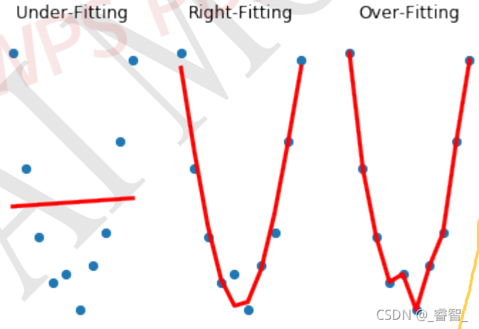
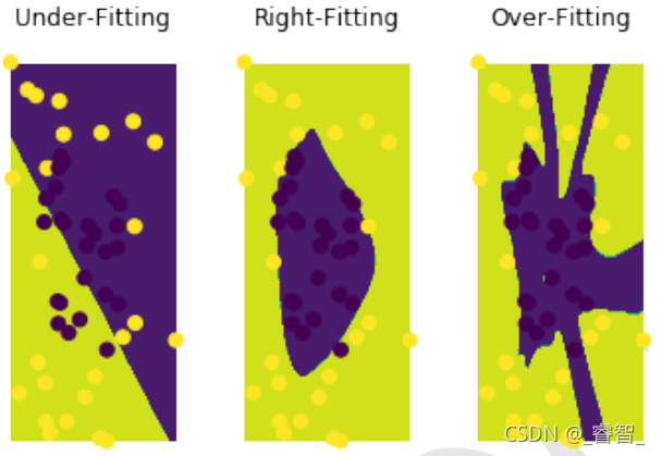
训练集中，过拟合的效果最好。

测试集中：

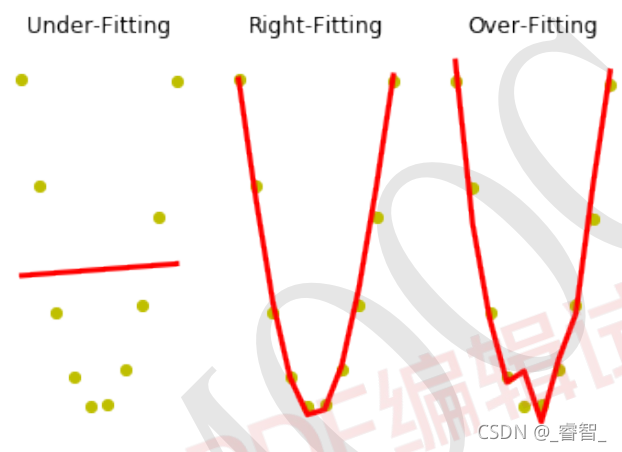
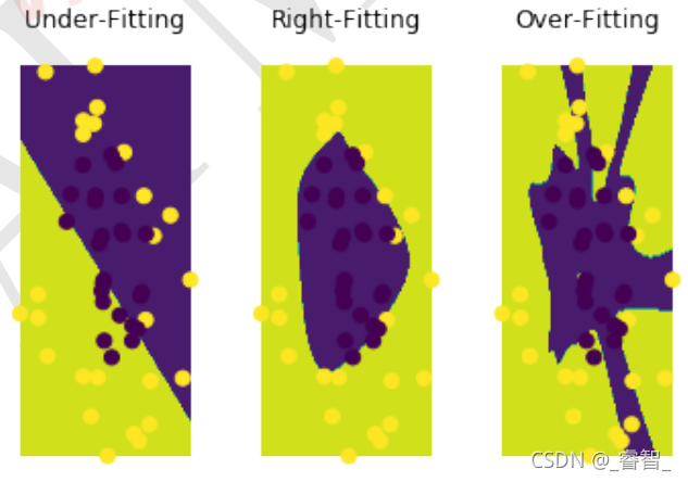
不难看出，测试集中是正确拟合的效果最好。

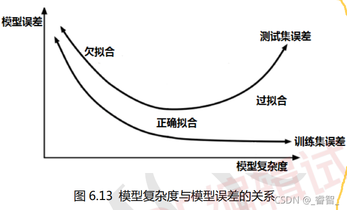
总结：过拟合虽然在训练集中的效果非常好，但是一旦到了测试集，效果就不如正确拟合好。

        模型复杂度在深度学习中主要指的是网络的层数以及每层网络神经元的各种，网络的层

数越多越复杂，神经元的个数越多越复杂。

        训练集的误差是随着模型复杂度的提升而不断降低的，测试集的误差是随着模型复杂度的提升而先下降后上升。

2、抵抗过拟合方法

增大数据集

提前停止(Early-Stopping)

Dropout

正则化

标签平滑(label Smoothing) 。

下面讲解一些过拟合处理方法：

过拟合处理（防止过拟合）：

一、数据增强

图像领域数据增强常用方式：

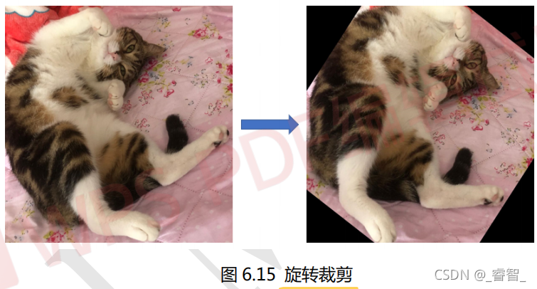
1、旋转/反射变换：随机旋转图像一定的角度，改变图像朝向。

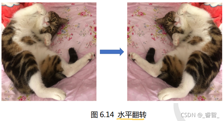
2、翻转变换：沿水平方向或竖直方向翻转图像。

3、缩放变换：按照一定的比例放大或缩小图像。

4、平移变换：在图像平面上对图像以一定方式平移。

5、尺度变换：对图像按照一定的尺度因子，进行放大或缩小。

6、对比度变换：在图像的HSV色彩空间中，保持色调H不变，改变饱和度S和亮度V，对每个像素的S和V分量进行指数运算。

7、噪声扰动：对图像的每个RGB随机噪声扰动。（噪声有：椒盐噪声、高斯噪声）

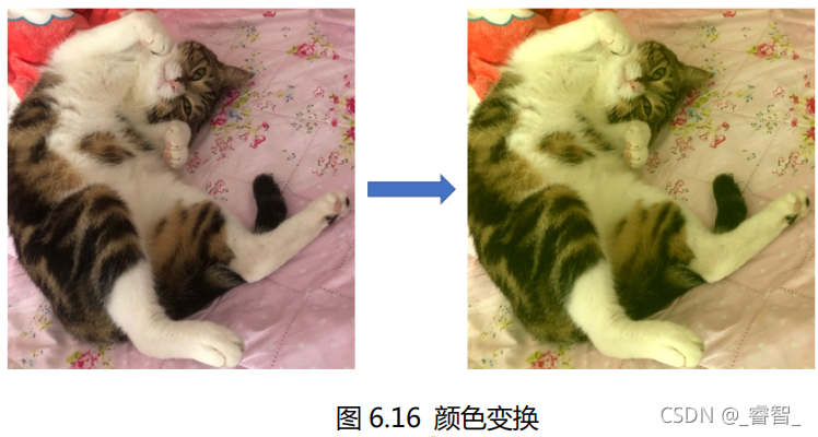
8、颜色变换：对图像的颜色进行一些有规律地调整。

 

步骤：

1、设置图像生成器

# 1、设置图像生成器
datagen = ImageDataGenerator(
    rotation_range = 40,            # 随机旋转度数
    width_shift_range = 0.2,        # 随机水平平移
    height_shift_range = 0.2,       # 随机竖直平移
    rescale = 1/255,                # 数据归一化
    shear_range = 30,               # 随机错切变换
    zoom_range = 0.2,               # 随机放大
    horizontal_flip = True,         # 水平翻转
    brightness_range = (0.7,1.3),   # 亮度变化
    fill_mode = 'nearest',)         # 填充方式

2、载入图片

# 2、载入图片
img = load_img('Resource/test11.jpg')

3、图像转三维数据

# 3、图像转三维数据(array:3维(height,width,channel))
img = img_to_array(img)

4、三维转四维

# 4、三维转四维（然后再做数据增强）
# 在第 0 个位置增加一个维度
# 4 维(1,height,width,channel)
img = np.expand_dims(img,0)

5、生成图片（用图像生成器）

# 5、生成20张图片
i = 0       # 生成的图片都保存在 images 文件夹中，文件名前缀为 new_image,图片格式为 jpeg
for batch in datagen.flow(img, batch_size=1, save_to_dir='images', save_prefix='new_image', save_format='jpeg'):
    i += 1
    if i==20:
        break

 得到这一系列的图像。

代码

# 图像数据增强
# 注：需要提前有一个文件夹（比如这里设置文件夹名为images，则需要提前准备一个images文件夹）
import os
os.environ['TF_CPP_MIN_LOG_LEVEL']='2'
 
from tensorflow.keras.preprocessing.image import ImageDataGenerator,img_to_array, load_img
import numpy as np
 
# 1、设置图像生成器
datagen = ImageDataGenerator(
    rotation_range = 40,            # 随机旋转度数
    width_shift_range = 0.2,        # 随机水平平移
    height_shift_range = 0.2,       # 随机竖直平移
    rescale = 1/255,                # 数据归一化
    shear_range = 30,               # 随机错切变换
    zoom_range = 0.2,               # 随机放大
    horizontal_flip = True,         # 水平翻转
    brightness_range = (0.7,1.3),   # 亮度变化
    fill_mode = 'nearest',         # 填充方式
)
 
# 2、载入图片
img = load_img('Resource/test11.jpg')
 
# 3、图像转三维数据(array:3维(height,width,channel))
img = img_to_array(img)
 
# 4、三维转四维（然后再做数据增强）
# 在第 0 个位置增加一个维度        4维:(1,height,width,channel)
img = np.expand_dims(img,0)
 
# 5、生成20张图片
i = 0       # 生成的图片都保存在 images 文件夹中，文件名前缀为 new_image,图片格式为 jpeg
for batch in datagen.flow(img, batch_size=1, save_to_dir='images', save_prefix='new_image', save_format='jpeg'):
    i += 1
    if i==20:
        break

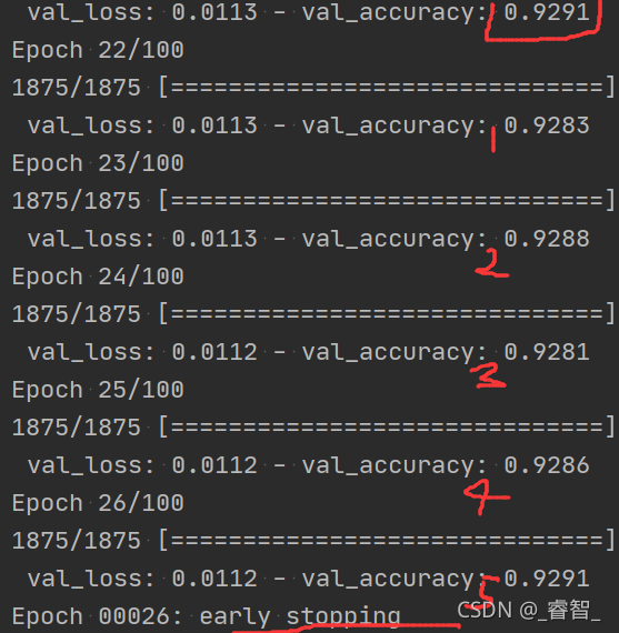
二、提前停止训练（Early-Stopping）

Early-Stopping 是一种 提前结束训练 的策略用来防止过拟合。

        训练效果不会随着迭代次数的增加无限提高 ， 记录到目前 为止最好的测试集准确率 p，之后连续 m 个周期没有超过最佳测试集准确率 p 时，则可以认 为 p 不再提高了，此时便可以提前停止迭代(Early-Stopping)。

1、设置回调函数（设置提前停止训练）

        设置val_accuracy为监测对象，记录每次的值，超过5次未超过之前的最佳值，则提前停止训练（早退）。

# 6、设置回调函数（提前停止训练）
early_stopping = EarlyStopping(monitor='val_accuracy', patience=5, verbose=1)
# monitor='val_accuracy'：监控验证集准确率
# patience=5：连续5个周期没有超过最高的val_accuracy值，则提前停止训练
# verbose=1：停止训练时提示 early stopping

2、训练（应用回调函数）

# 7、训练（应用回调函数）
model.fit(train_data, train_label, epochs=100, batch_size=32, validation_data=(test_data, test_label),
callbacks=[early_stopping])
# 回调函数（提前停止训练）

效果：

 

代码

# 提前停止训练（Early_Callback）
import os
os.environ['TF_CPP_MIN_LOG_LEVEL']='2'
 
import tensorflow as tf
from tensorflow.keras.optimizers import SGD
from tensorflow.keras.callbacks import EarlyStopping
 
# 1、载入数据集
mnist = tf.keras.datasets.mnist
(train_data, train_label), (test_data, test_label) = mnist.load_data()
 
# 2、归一化处理（有助于提升模型训练速度）
train_data, test_data = train_data / 255.0, test_data / 255.0
 
# 3、独热编码
train_label = tf.keras.utils.to_categorical(train_label,num_classes=10)
test_label = tf.keras.utils.to_categorical(test_label,num_classes=10) # 模型定义
 
# 4、搭建神经网络
model = tf.keras.models.Sequential([
tf.keras.layers.Flatten(input_shape=(28, 28)),  #数据压缩（三维->二维：(60000,28,28)->(60000,784)
tf.keras.layers.Dense(10, activation='softmax')
])
 
# 5、设置优化器、损失函数、标签
model.compile(optimizer=SGD(0.5), loss='mse', metrics=['accuracy'])
# EarlyStopping 是 Callbacks 的一种，callbacks用于指定在每个epoch或batch开始和结束的时候进行哪种特定操作
 
# 6、设置回调函数（提前停止训练）
early_stopping = EarlyStopping(monitor='val_accuracy', patience=5, verbose=1)
# monitor='val_accuracy'：监控验证集准确率
# patience=5：连续5个周期没有超过最高的val_accuracy值，则提前停止训练
# verbose=1：停止训练时提示 early stopping
 
# 7、训练（应用回调函数）
model.fit(train_data, train_label, epochs=100, batch_size=32, validation_data=(test_data, test_label),
callbacks=[early_stopping])
# 回调函数（提前停止训练）

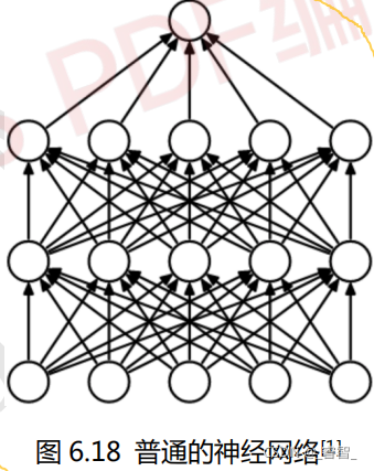
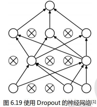
三、Dropout

1、搭建神经网络进行对比

1-1、普通神经网络

# 4、搭建神经网络（normal）
model = Sequential([
Flatten(input_shape=(28, 28)),
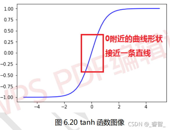
Dense(units=200,activation='tanh'),
Dense(units=100,activation='tanh'),
Dense(units=10,activation='softmax')
])

1-2、dropout神经网络

# 4、搭建神经网络（Dropout）
model_dropout = Sequential([
Flatten(input_shape=(28, 28)),
Dense(units=200,activation='tanh'),
Dropout(0.4),
Dense(units=100,activation='tanh'),
Dropout(0.4),
Dense(units=10,activation='softmax')
])

2、训练

# 6、训练
# 先训练正常模型
history1 = model.fit(train_data, train_target, epochs=30, batch_size=32, validation_data=(test_data, test_target))
 
# 再训练Dropout模型
history2 = model_dropout.fit(train_data, train_target, epochs=30, batch_size=32, validation_data=(test_data, test_target))

3、画图

# 7、画图
# 画出 model1 验证集准确率曲线图
plt.plot(np.arange(30), normal_history.history['val_accuracy'], c='b', label='normal')
plt.plot(np.arange(30), dropout_history.history['val_accuracy'], c='y', label='dropout')
#       横坐标(0~30)     获取训练结果                               颜色    标签
plt.legend()
 
# x 坐标描述
plt.xlabel('epochs')
# y 坐标描述
plt.ylabel('accuracy')
 
# 显示图像
plt.show()

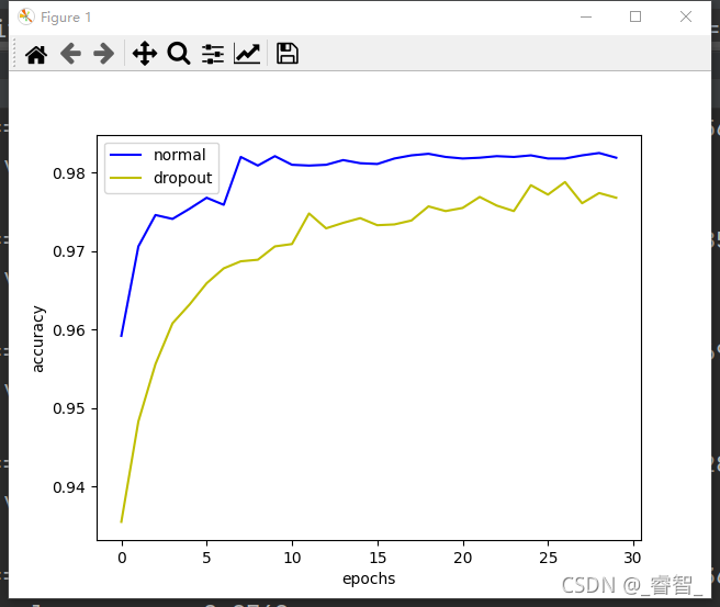
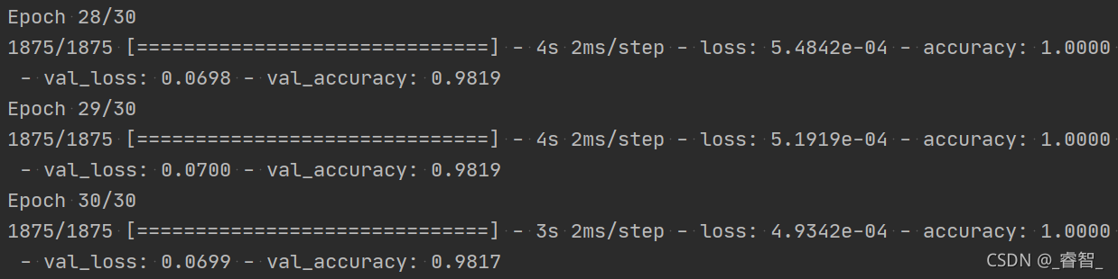
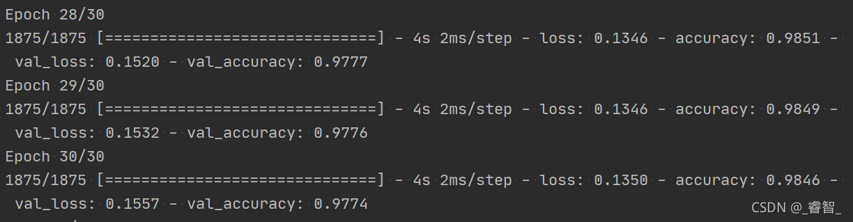
normal：

 dropout：

        可以发现dropout的测试集正确率甚至比正确率还要高，这是因为：模型在训练的时候使用了dropout，但是在测试集的时候没有使用dropout。

        这里训练的次数比较少，如果训练更多的次数，那么dropout的测试集准确率将达到98.8%，比normal的测试集准确率还要高（98,2%）

代码

# Dropout
import os
os.environ['TF_CPP_MIN_LOG_LEVEL']='2'
 
import tensorflow as tf
from tensorflow.keras.models import Sequential
from tensorflow.keras.layers import Dense,Dropout,Flatten
from tensorflow.keras.optimizers import SGD
import matplotlib.pyplot as plt
import numpy as np
 
# 1、载入数据集
mnist = tf.keras.datasets.mnist
(train_data, train_target), (test_data, test_target) = mnist.load_data()
 
# 2、归一化处理（有助于提升模型训练速度）
train_data, test_data = train_data / 255.0, test_data / 255.0
 
# 3、独热编码
train_target = tf.keras.utils.to_categorical(train_target,num_classes=10)
test_target = tf.keras.utils.to_categorical(test_target,num_classes=10) # 模型定义，model1 使用 Dropout
# Dropout(0.4)表示隐藏层 40%神经元不工作
 
# 4、搭建神经网络（normal）
model = Sequential([
Flatten(input_shape=(28, 28)),
Dense(units=200,activation='tanh'),
Dense(units=100,activation='tanh'),
Dense(units=10,activation='softmax')
])
 
# 4、搭建神经网络（Dropout）
model_dropout = Sequential([
Flatten(input_shape=(28, 28)),
Dense(units=200,activation='tanh'),
Dropout(0.4),
Dense(units=100,activation='tanh'),
Dropout(0.4),
Dense(units=10,activation='softmax')
])
 
# 5、设置优化器、损失、标签
model.compile(optimizer=SGD(0.2), loss='categorical_crossentropy', metrics=['accuracy'])
model_dropout.compile(optimizer=SGD(0.2), loss='categorical_crossentropy', metrics=['accuracy'])
 
# 6、训练
# 先训练正常模型
normal_history = model.fit(train_data, train_target, epochs=30, batch_size=32, validation_data=(test_data, test_target))
 
# 再训练Dropout模型
dropout_history = model_dropout.fit(train_data, train_target, epochs=30, batch_size=32, validation_data=(test_data, test_target))
 
# 7、画图
# 画出 model1 验证集准确率曲线图
plt.plot(np.arange(30), normal_history.history['val_accuracy'], c='b', label='normal')
plt.plot(np.arange(30), dropout_history.history['val_accuracy'], c='y', label='dropout')
#       横坐标(0~30)     获取训练结果                               颜色    标签
plt.legend()
 
# x 坐标描述
plt.xlabel('epochs')
# y 坐标描述
plt.ylabel('accuracy')
 
# 显示图像
plt.show()

四、正则化

        L1 和 L2 正则化的使用实际上就是在普通的代价函数（例如均方差代价函数或交叉熵代价函数）后面加上一个正则项。最小化正则项的值，实际上就是让w的值接近于0。

1、L1正则化

加上了L1正则项的交叉熵：

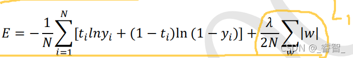
2、L2正则化

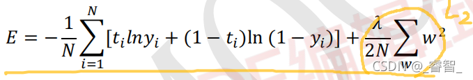
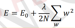
当w变得很小之后，wx+b的计算会变成一个接近0的值：

         正则化使得神经网络中增加了很多线性特征，减少了很多非线性特征，网络复杂度降低，所以不容易出现过拟合。

步骤：

1、神经网络中添加正则化操作

设置L2正则化，正则化系数：0.0003。 

# 4、神经网络（正则化：正则化系数：0.0003）
model_l2 = Sequential([
Flatten(input_shape=(28, 28)),
Dense(units=200,activation='tanh',kernel_regularizer=l2(0.0003)),
Dense(units=100,activation='tanh',kernel_regularizer=l2(0.0003)),
Dense(units=10,activation='softmax',kernel_regularizer=l2(0.0003))
])

2、编译

# 5、设置优化器、损失函数、标签
model_l2.compile(optimizer=SGD(0.2), loss='categorical_crossentropy', metrics=['accuracy'])
model.compile(optimizer=SGD(0.2), loss='categorical_crossentropy', metrics=['accuracy'])
# categorical_crossentropy：交叉熵损失函数

3、训练

# 6、训练
# 先训练 model_l2
history_l2 = model_l2.fit(train_data, train_target, epochs=30, batch_size=32, validation_data=(test_data,test_target))
# 再训练 model
history = model.fit(train_data, train_target, epochs=30, batch_size=32, validation_data=(test_data,test_target))

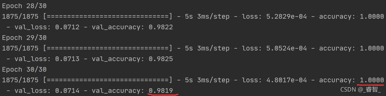
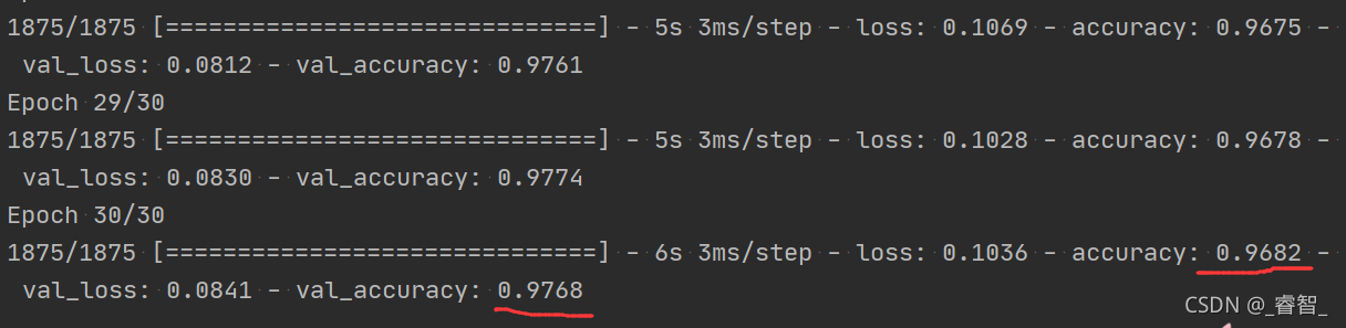
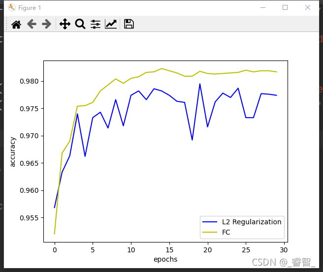
效果：

正常：

L2正则化：

代码

# L2正则化
import os
os.environ['TF_CPP_MIN_LOG_LEVEL']='2'
 
import tensorflow as tf
from tensorflow.keras.models import Sequential
from tensorflow.keras.layers import Dense,Dropout,Flatten
from tensorflow.keras.optimizers import SGD
import matplotlib.pyplot as plt
import numpy as np
# 使用 l1 或 l2 正则化
from tensorflow.keras.regularizers import l1,l2
 
# 1、载入数据
mnist = tf.keras.datasets.mnist
(train_data, train_target), (test_data, test_target) = mnist.load_data()
 
# 2、归一化处理（有助于提升模型训练速度）
train_data, test_data = train_data / 255.0, test_data / 255.0
 
# 3、独热编码
train_target = tf.keras.utils.to_categorical(train_target,num_classes=10)
test_target = tf.keras.utils.to_categorical(test_target,num_classes=10) # 模型定义，model_l2 使用 l2 正则化 # l2(0.0003)表示使用 l2 正则化，正则化系数为 0.0003
 
# 4、神经网络（正则化：正则化系数：0.0003）
model_l2 = Sequential([
Flatten(input_shape=(28, 28)),
Dense(units=200,activation='tanh',kernel_regularizer=l2(0.0003)),
Dense(units=100,activation='tanh',kernel_regularizer=l2(0.0003)),
Dense(units=10,activation='softmax',kernel_regularizer=l2(0.0003))
])
 
# 神经网络（正常，无正则化）
model = Sequential([
Flatten(input_shape=(28, 28)),
Dense(units=200,activation='tanh'),
Dense(units=100,activation='tanh'),
Dense(units=10,activation='softmax')
])
 
# 5、设置优化器、损失函数、标签
model_l2.compile(optimizer=SGD(0.2), loss='categorical_crossentropy', metrics=['accuracy'])
model.compile(optimizer=SGD(0.2), loss='categorical_crossentropy', metrics=['accuracy'])
# categorical_crossentropy：交叉熵损失函数
 
# 6、训练
# 先训练 model_l2
history_l2 = model_l2.fit(train_data, train_target, epochs=30, batch_size=32, validation_data=(test_data,test_target))
# 再训练 model
history = model.fit(train_data, train_target, epochs=30, batch_size=32, validation_data=(test_data,test_target))
 
# 7、画图
plt.plot(np.arange(30),history_l2.history['val_accuracy'], c='b',label='L2 Regularization') # 画出 model 验证集准确率曲线图
plt.plot(np.arange(30),history.history['val_accuracy'], c='y',label='FC') # 图例
plt.legend()
 
# x 坐标描述
plt.xlabel('epochs')
# y 坐标描述
plt.ylabel('accuracy')
# 显示图像
plt.show()

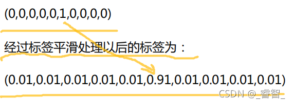
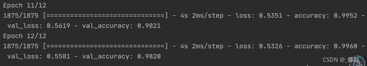
五、标签平滑

标签平滑（LSR）：也称为标签平滑正则化。 

例：

 

1、在损失函数中定义平滑系数

# 定义交叉熵函数（设置平滑系数）
loss = CategoricalCrossentropy(label_smoothing=0)
loss_smooth = CategoricalCrossentropy(label_smoothing=0.1)
# label_smoothing：平滑系数

2、编译

# 编译
model.compile(optimizer=SGD(0.2), loss=loss, metrics=['accuracy'])
model_smooth.compile(optimizer=SGD(0.2), loss=loss_smooth, metrics=['accuracy'])

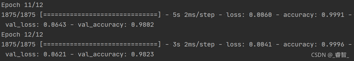
3、训练

# 6、训练
# 先训练 model
history = model.fit(train_data, train_target, epochs=12, batch_size=32, validation_data=(test_data,test_target))
# 再训练 model_smooth
history_smooth = model_smooth.fit(train_data, train_target, epochs=12, batch_size=32, validation_data=(test_data,test_target))

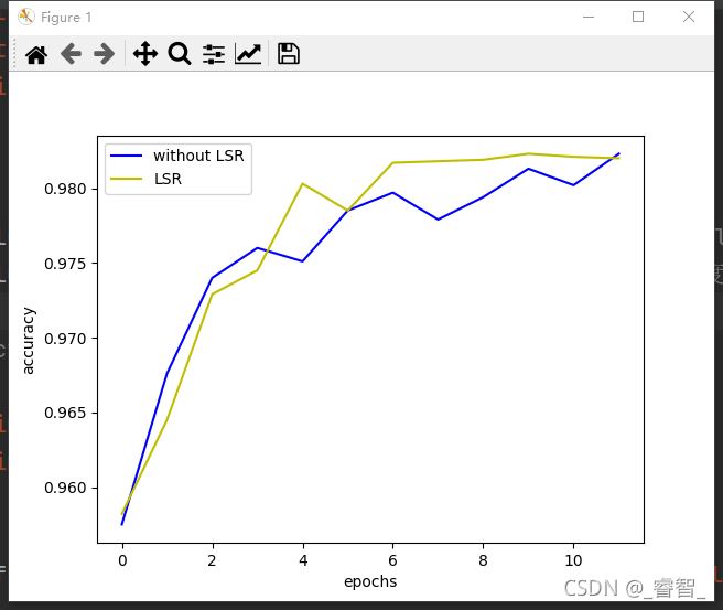
效果： 

 

代码

# 标签平滑
import os
os.environ['TF_CPP_MIN_LOG_LEVEL']='2'
 
import tensorflow as tf
from tensorflow.keras.models import Sequential
from tensorflow.keras.layers import Dense,Dropout,Flatten
from tensorflow.keras.optimizers import SGD
from tensorflow.keras.losses import CategoricalCrossentropy
import matplotlib.pyplot as plt
import numpy as np
 
# 1、载入数据
mnist = tf.keras.datasets.mnist
(train_data, train_target), (test_data, test_target) = mnist.load_data()
 
# 2、归一化处理（有助于提升模型训练速度）
train_data, test_data = train_data / 255.0, test_data / 255.0
 
# 3、独热编码
train_target = tf.keras.utils.to_categorical(train_target,num_classes=10)
test_target = tf.keras.utils.to_categorical(test_target,num_classes=10) # 模型定义，model 不用 label smoothing
 
# 4、神经网络（普通）
model = Sequential([
    Flatten(input_shape=(28, 28)),
    Dense(units=200,activation='tanh'),
    Dense(units=100,activation='tanh'),
    Dense(units=10,activation='softmax')
])
 
# 神经网络（标签平滑）
model_smooth = Sequential([
Flatten(input_shape=(28, 28)),
Dense(units=200,activation='tanh'),
Dense(units=100,activation='tanh'),
Dense(units=10,activation='softmax')
])
 
# 5、编译
# 定义交叉熵函数（设置平滑系数）
loss = CategoricalCrossentropy(label_smoothing=0)
loss_smooth = CategoricalCrossentropy(label_smoothing=0.1)
# label_smoothing：平滑系数
# 编译
model.compile(optimizer=SGD(0.2), loss=loss, metrics=['accuracy'])
model_smooth.compile(optimizer=SGD(0.2), loss=loss_smooth, metrics=['accuracy'])
 
# 6、训练
# 先训练 model
history = model.fit(train_data, train_target, epochs=12, batch_size=32, validation_data=(test_data,test_target))
# 再训练 model_smooth
history_smooth = model_smooth.fit(train_data, train_target, epochs=12, batch_size=32, validation_data=(test_data,test_target))
 
# 7、画图
plt.plot(np.arange(12),history.history['val_accuracy'],c='b',label='without LSR') # 画出 model_smooth 验证集准确率曲线图
plt.plot(np.arange(12),history_smooth.history['val_accuracy'],c='y',label='LSR') # 图例
plt.legend()
# x 坐标描述
plt.xlabel('epochs')
# y 坐标描述
plt.ylabel('accuracy')
# 显示图像
plt.show()