基于卷积神经网络的高光谱图像分类详细教程（含python代码）_支持向量机怎么实现高光谱分类

目录

一、背景

二、基于卷积神经网络的代码实现

1）建立卷积神经网络模型

2）训练函数代码

3）全图可视化

三、项目代码

---

一、背景

卷积神经网络（Convolutional Neural Networks, CNNs）在处理高光谱图像分类任务时，展现出了卓越的性能。高光谱图像因其丰富的光谱信息而具有极高的空间分辨率，能够捕捉到物体在不同波段上的细微差异。CNNs通过其特有的卷积层、池化层和全连接层结构，能够自动提取图像中的空间和光谱特征，有效地捕捉到高光谱数据中的复杂模式。在卷积层中，局部感受野和权值共享机制使得网络能够学习到图像的局部特征，而池化层则有助于减少参数数量，提高特征的不变性。通过层层堆叠的非线性变换，CNNs能够构建出深层次的特征表示，从而实现对高光谱图像中不同地物类别的高精度分类。此外，通过引入迁移学习、数据增强和正则化等技术，可以进一步提高模型的泛化能力和分类性能，使得卷积神经网络成为高光谱图像分析领域的一项重要工具。

深度学习是机器学习的一个分支，它通过构建多层的神经网络来模拟人脑处理信息的方式，从而实现对复杂数据的高效处理和模式识别。在深度学习中，2D卷积是一种核心操作，尤其在图像处理和计算机视觉领域中扮演着至关重要的角色。

2D卷积操作涉及一个卷积核（或滤波器），它在输入数据（如图像）上滑动，计算卷积核与输入数据局部区域的点积，从而生成输出特征图。这个过程可以捕捉到输入数据的空间层次结构，即从低级特征（如边缘和角点）到高级特征（如纹理和对象部分）的逐步抽象。

二、基于卷积神经网络的代码实现

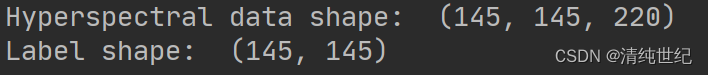
下面我们以IP数据集为例子进行展开讲解。

1）建立卷积神经网络模型

import torch.nn as nn
 
class CNN_2D(nn.Module):
    def __init__(self, num_classes):
        super(CNN_2D, self).__init__()
        # 2D卷积块
        self.block_2D = nn.Sequential(
            nn.Conv2d(
                in_channels=30,out_channels=64,kernel_size=(3, 3),stride=(2,2),padding=(1,1)),
            nn.ReLU(inplace=True),
            nn.Conv2d(in_channels=64,out_channels=128,kernel_size=(3, 3),stride=(2,2),padding=(1,1)),
            nn.ReLU(inplace=True),
            nn.Conv2d(in_channels=128,out_channels=256,kernel_size=(3, 3),stride=(2,2),padding=(1,1)),
            nn.ReLU(inplace=True)
        )
 
        # 全连接层
        self.classifier = nn.Sequential(
            nn.Linear(in_features=16*256,out_features=512
            ),
            nn.Dropout(p=0.4),
            nn.Linear(in_features=512,out_features=256
            ),
            nn.Dropout(p=0.4),
            nn.Linear(in_features=256,out_features=num_classes))
 
    def forward(self, x):
        y = self.block_2D(x)
        y = y.reshape(y.shape[0], -1)
        y = self.classifier(y)
        return y

2）训练函数代码

1、导入相关包

首先导入训练需要用到的相关函数和包

from utils import applyPCA,createImageCubes,splitTrainTestSet,reports
import scipy.io as sio
from net import CNN_2D
import torch
import numpy as np
import os
import torch.nn as nn
import torch.optim as optim
import matplotlib.pyplot as plt
import time

2、数据集加载

将下载的数据加载进内存，便于后续处理

X = sio.loadmat('./data/Indian_pines.mat')['indian_pines']
y = sio.loadmat('./data/Indian_pines_gt.mat')['indian_pines_gt']

3、PCA降维

由于数据的波段非常大，这里利用PCA进行数据降维。降维后数据维度得到减少，从220个波段降维到30个波段。

X_pca = applyPCA(X, numComponents=pca_components)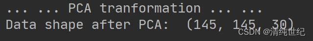

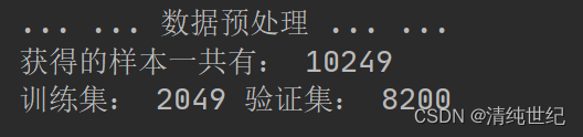
4、数据集的样本划分与标签分配

根据数据标签和数据，对其进行样本采样，并划分成训练集和验证集。这里以窗口为25的大小，训练集和测试集的占比分别为20%的训练，80%的验证。

X_pca, y = createImageCubes(X_pca, y, windowSize=patch_size)
Xtrain, Xtest, ytrain, ytest = splitTrainTestSet(X_pca, y, test_ratio)

5、转数据为torch张量

首先定义样本加载函数：

# 加载数据函数
class TrainDS(torch.utils.data.Dataset):
    def __init__(self):
        self.len = Xtrain.shape[0]
        self.x_data = torch.FloatTensor(Xtrain)
        self.y_data = torch.LongTensor(ytrain)
    def __getitem__(self, index):
        # 根据索引返回数据和对应的标签
        return self.x_data[index], self.y_data[index]
    def __len__(self):
        # 返回文件数据的数目
        return self.len
 
class TestDS(torch.utils.data.Dataset):
    def __init__(self):
        self.len = Xtest.shape[0]
        self.x_data = torch.FloatTensor(Xtest)
        self.y_data = torch.LongTensor(ytest)
    def __getitem__(self, index):
        # 根据索引返回数据和对应的标签
        return self.x_data[index], self.y_data[index]
    def __len__(self):
        # 返回文件数据的数目
        return self.len

然后将数据以批量的方式加载进来：

trainset = TrainDS()
testset  = TestDS()
train_loader = torch.utils.data.DataLoader(dataset=trainset, batch_size=128, shuffle=True)
test_loader  = torch.utils.data.DataLoader(dataset=testset,  batch_size=128, shuffle=False)

6、自动选择GPU还是CPU训练

# 使用GPU训练
device = torch.device("cuda:0" if torch.cuda.is_available() else "cpu")
# 网络放到GPU上
net = CNN_2D(num_classes=class_num).to(device)

7、设置相关的损失、优化函数以及迭代次数

EPOCH = 10
criterion = nn.CrossEntropyLoss()
optimizer = optim.Adam(net.parameters(), lr=0.001)

8、开始训练

训练过程中，保存验证集最优结果的权值，以便后续使用。

for epoch in range(EPOCH):
    for i, (inputs, labels) in enumerate(train_loader):
        inputs = inputs.to(device)
        labels = labels.to(device)
        optimizer.zero_grad()
        outputs = net(inputs)
        loss = criterion(outputs, labels)
        loss.backward()
        optimizer.step()

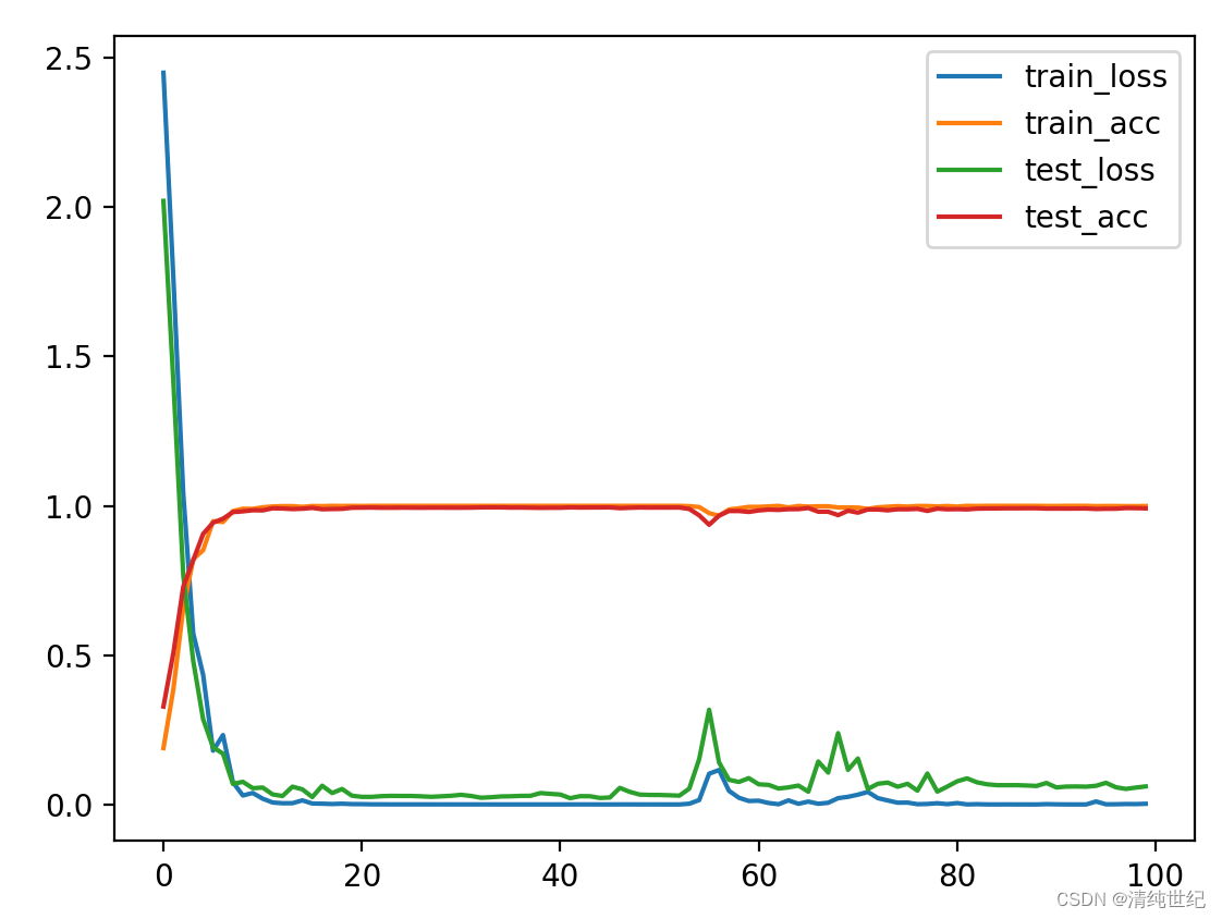
9、绘制损失和准确率曲线

将训练过程中的损失和准确率保存，并进行绘制，查看他们之间的关系。

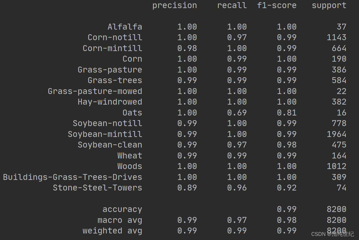
10、对验证集进行评估，获取最终结果

classification, confusion, oa, each_acc, aa, kappa, names = reports(ytest, y_pred_test)
print(classification)
print("混淆矩阵\n",confusion)
print("kapap:", kappa)
print("aa:", aa)
print("oa:", oa)
print("训练时间：",train_time_1-train_time_0,"验证时间：",test_time_1-test_time_0)

3）全图可视化

采用逐点预测的方式

for i in range(height):
    for j in range(width):
        image_patch = X[i:i+patch_size, j:j+patch_size, :]
        image_patch = image_patch.reshape(1,image_patch.shape[0],image_patch.shape[1], image_patch.shape[2])
        X_test_image = torch.FloatTensor(image_patch.transpose(0, 3, 1, 2)).to(device)
        prediction = net(X_test_image)
        prediction = np.argmax(prediction.detach().cpu().numpy(), axis=1)
        outputs[i][j] = prediction+1

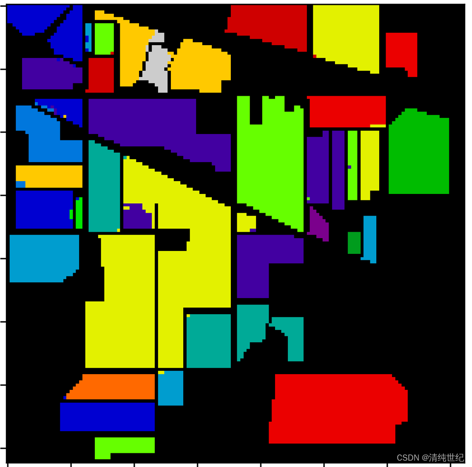
预测结果比较不错，精度99%以上了。

三、项目代码

本项目的代码通过以下链接下载：基于卷积神经网络的高光谱图像分类代码