sklearn实现逻辑回归_以python为工具【Python机器学习系列（十）】_python逻辑回归模型from sklearn_sklearn非线性回归

---

第三步，训练模型

logistic = LogisticRegression()
logistic.fit(x_data, y_data)

# 截距
print(logistic.intercept_)
# 系数：theta1 theta2
print(logistic.coef_)
# 预测
pred = logistic.predict(x_data)
# 输出评分
score = logistic.score(x_data, y_data)
print(score)

1
2
3
4
5
6
7
8
9
10
11
12
13

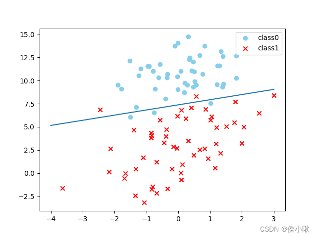
输出结果如下图所示：
        

---

绘制出带有决策边界的散点图：

# 绘制散点
plot_logi()
# 绘制决策边界
x_test = np.array([[-4], [3]])
y_test = -(x_test\*logistic.coef_[0, 0]+logistic.intercept_)/logistic.coef_[0, 1]
plt.plot(x_test, y_test)
plt.show()

1
2
3
4
5
6
7
8

---

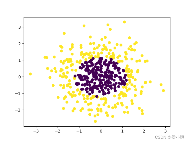
2.非线性逻辑回归

python实现非线性逻辑回归，首先使用make_gaussian_quantiles获取一组高斯分布的数据集，代码及数据分布如下：

import matplotlib.pyplot as plt
from sklearn import linear_model
from sklearn.preprocessing import PolynomialFeatures
from sklearn.datasets import make_gaussian_quantiles


# 获取高斯分布的数据集，500个样本，2个特征，2分类
x_data, y_data = make_gaussian_quantiles(n_samples=500, n_features=2, n_classes=2)
# 绘制散点图
plt.scatter(x_data[:, 0], x_data[:, 1],c=y_data)
plt.show()

1
2
3
4
5
6
7
8
9
10
11
12

描述数据分布的散点图如图所示：
        

---

然后转换数据并训练模型以实现非线性逻辑回归：

# 数据转换，最高次项为五次项
poly_reg = PolynomialFeatures(degree=5)
x_poly = poly_reg.fit_transform(x_data)


# 定义逻辑回归模型
logistic = linear_model.LogisticRegression()
logistic.fit(x_poly, y_data)
score = logistic.score(x_poly, y_data)
print(score)

1
2
3
4
5
6
7
8
9
10
11

评分结果如图所示，达0.996：
        

---

3.乳腺癌数据集案例

以乳腺癌数据集为例，建立线性逻辑回归模型，并输出准确率，精确率，召回率三大指标，代码如下所示：

from sklearn.datasets import load_breast_cancer
from sklearn.linear_model import LogisticRegression
from sklearn.model_selection import train_test_split
from sklearn.metrics import recall_score
from sklearn.metrics import precision_score
from sklearn.metrics import classification_report
from sklearn.metrics import accuracy_score
import warnings

warnings.filterwarnings("ignore")

# 获取数据
cancer = load_breast_cancer()
# 分割数据
X_train, X_test, y_train, y_test = train_test_split(cancer.data, cancer.target, test_size=0.2)

# 创建估计器
model = LogisticRegression()
# 训练
model.fit(X_train, y_train)

# 训练集准确率
train_score = model.score(X_train, y_train)
# 测试集准确率
test_score = model.score(X_test, y_test)
print('train score:{train\_score:.6f};test score:{test\_score:.6f}'.format(train_score=train_score, test_score=test_score))
print("==================================================================================")
# 再对X\_test进行预测
y_pred = model.predict(X_test)
print(y_pred)
# 准确率 所有的判断中有多少判断正确的
accuracy_score_value = accuracy_score(y_test, y_pred)
# 精确率 预测为正的样本中有多少是对的
precision_score_value = precision_score(y_test, y_pred)
# 召回率 样本中有多少正样本被预测正确了
recall_score_value = recall_score(y_test, y_pred)

print("准确率：", accuracy_score_value)
print("精确率：", precision_score_value)
print("召回率：", recall_score_value)

# 输出报告模型评估报告
classification_report_value = classification_report(y_test, y_pred)

print(classification_report_value)

1
2
3
4
5
6
7
8
9
10
11
12
13
14
15
16
17
18
19
20
21
22
23
24
25
26
27
28
29
30
31
32
33
34
35
36
37
38
39
40
41
42
43
44
45
46

程序输出结果如下图所示：

---

本次分享就到这里，小啾感谢您的关注与支持！
本文内容由网友自发贡献，转载请注明出处：https://www.wpsshop.cn/w/小桥流水78/article/detail/748020