Swin Transformer V2（CVPR 2022）论文与代码解读_swin transformerv2

paper：Swin Transformer V2: Scaling Up Capacity and Resolution

official implementation：https://github.com/microsoft/Swin-Transformer

third-party implementation：https://github.com/huggingface/pytorch-image-models/blob/main/timm/models/swin_transformer_v2.py

存在的问题

大规模视觉模型在训练和应用过程中存在三个主要问题：

1. 训练的不稳定性：大模型在训练过程中存在激活幅度差异过大的问题。
2. 预训练和微调之间的分辨率差异：高分辨率任务与低分辨率预训练之间的分辨率差异。
3. 对标注数据的需求：大规模模型需要大量标注数据进行训练。

本文的创新点

针对上述三个问题，本文提出了三种对应的解决方法：

1. residual-post-norm and cosine attention：在模型架构中引入残差后规范化方法和余弦注意力机制，提高了大模型的训练稳定性和准确性。
2. log-spaced continuous position bias（Log-CPB）：这种新方法允许模型在不同窗口大小之间自由转移，解决了高低分辨率任务之间的迁移问题。
3. 自监督预训练方法（SimMIM）：通过自监督学习减少对标注数据的需求，使得训练过程更加高效。

方法介绍

当扩大Swin Transformer的模型容量和窗口大小时作者观察到了两个问题：

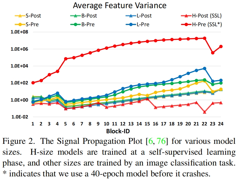
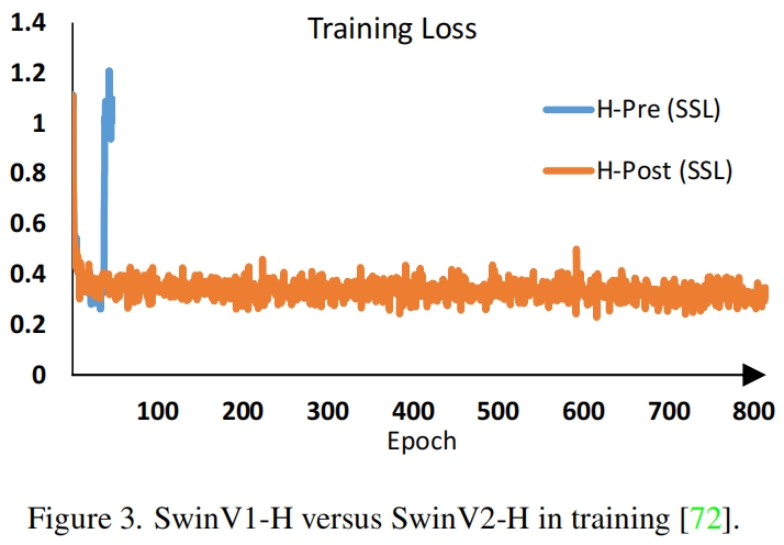
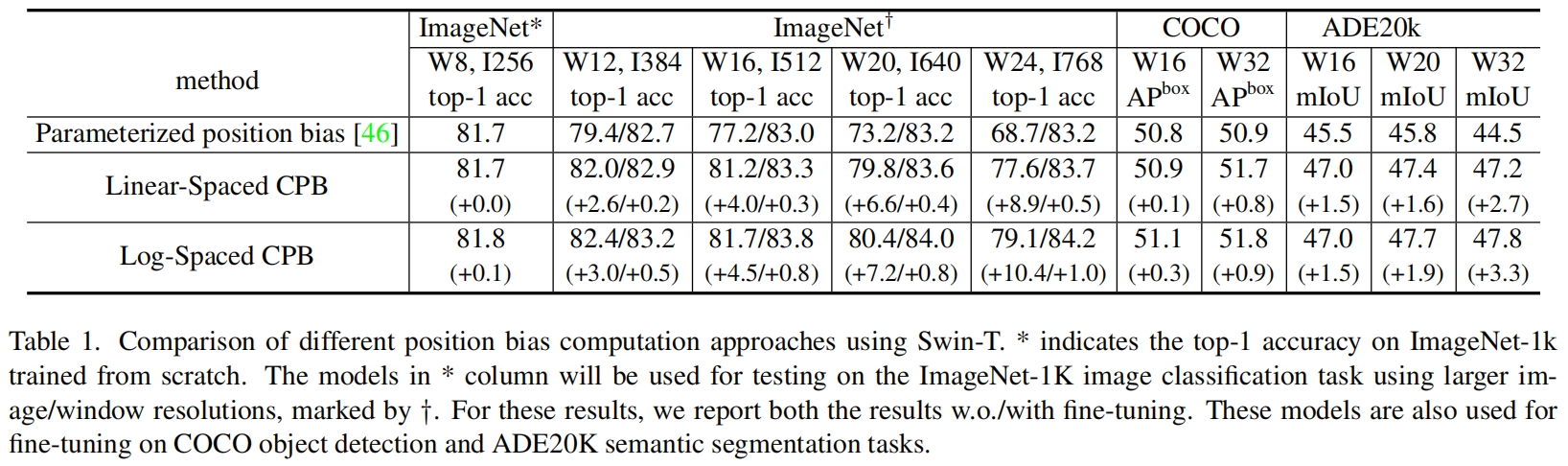
• 当扩大模型容量时出现的不稳定问题。如图2所示，当我们将原始的Swin Transformer从小尺寸扩大到大尺寸时，深层的激活值明显增大。最大值与最小值之间的差异达到了 $10^4$。当进一步增大模型尺寸（6.58亿个参数）时，模型无法收敛，如图3所示。
• 当迁移模型时窗口大小不同，性能下降明显。如表1第一行所示，当通过bi-cubic插值在更大的输入分辨率和更大的窗口尺寸下直接测试一个在ImageNet-1K上训练的模型（输入大小256x256，窗口大小8x8）时，精度下降明显。因此有必要重新研究Swin Transformer中的相对位置偏差。

在原始的Swin Transformer中，每个block的开始都有一个layer norm层，在这种pre-normalization设置下，每个residual block的输出值被直接合并回主分支，因此主分支的值随着网络层的加深变得原来越大。不同层激活值过大的差异导致训练的不稳定性。

Post normalization

为了缓解这个问题，作者提出了使用residual post normalization方法，如图1所示。

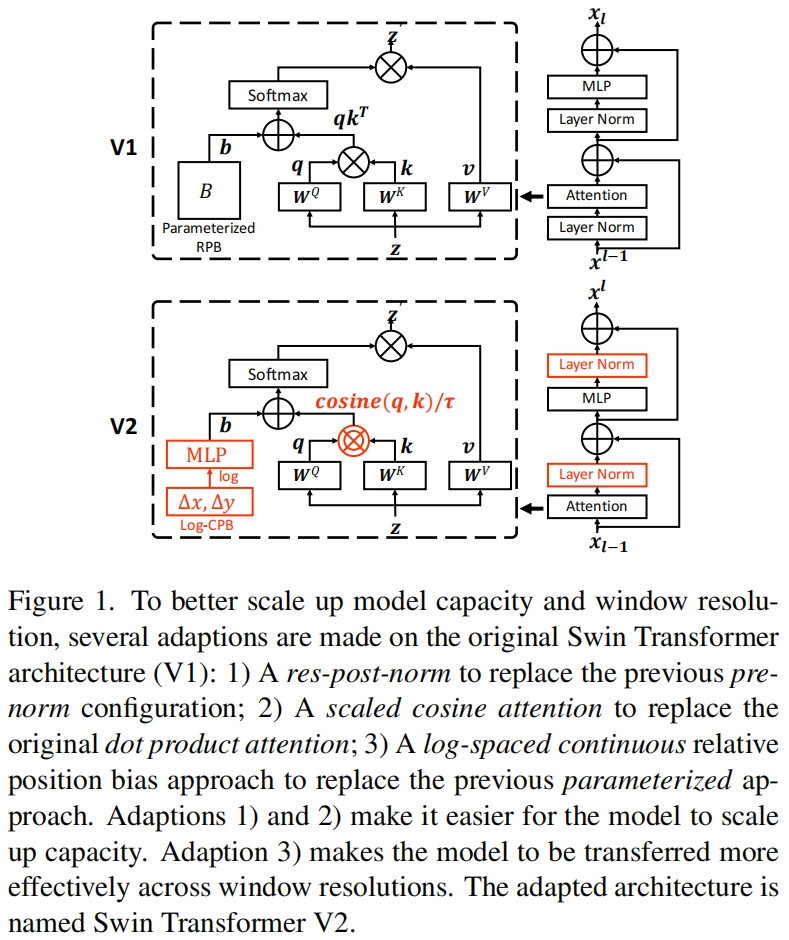
在这种方法中，每个残差块的输出在被合并回主分支前进行归一化，随着网络变深，主分支的振幅不会累积。如图2所示，这种方法的激活振幅比原始的pre-normalization要温和的多。在本文最大模型的训练中，作者在每6个transformer block的主分支上额外添加一个layer normalization层，以进一步稳定训练。 

Scaled cosine attention

在原始的self-attention计算中，用query和key向量的点积来衡量像素点之间的相似度。作者发现，当这种方法用于大型视觉模型时，一些block和head学习到的attention map经常被少数像素对所主导，特别是在res-post-norm配置下。为了缓解这个问题，作者提出了一种缩放余弦注意力方法，通过scaled cosine函数来计算像素对 $i$ 和 $j$ 之间的注意力

其中 $B_{ij}$ 是像素 $i$ 和 $j$ 的相对位置偏差，$\tau$ 是一个可学习的标量，在不同的heads和layer之间不共享，且值设置为大于0.01。余弦函数本身就是归一化的，因此可以得到一个较温和的注意力值。

Continuous relative position bias

和原始的Swin Transformer中直接优化参数化的偏差不同，本文提出的连续相对位置偏差方法在相对坐标上用了一个小的网络来学习

其中 $\mathcal{G}$ 是一个小网络，默认是一个两层的MLP，中间有一个ReLU激活函数。网络 $\mathcal{G}$ 为任意的相对坐标生成bias值，因此可以很自然地迁移到具有任意窗口大小的微调任务中。在推理时，可以预先计算每个相对位置的偏差值，并作为模型的参数存储，从而和原始的直接学习的参数化的bias方法相同。

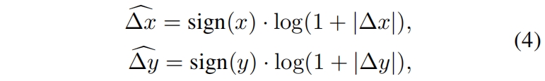
Log-spaced coordinates

当迁移到窗口大小变化很大的任务中时，需要extrapolate推算很大范围的相对坐标。为了缓解这个问题，作者提出log-spaced对数间隔的坐标，而不是原来的linear-spaced线性间隔的坐标。

其中 $\Delta x,\Delta y$ 和 $\widehat{\Delta x}, \widehat{\Delta y}$ 分别是线性间隔和对数间隔的坐标。

通过使用对数间隔坐标，当我们在不同窗口分辨率之间迁移相对位置偏差时，所需的extrapolation ratio外推比将比使用原始的线性间隔坐标要小得多。比如当从一个预训练的8x8窗口大小迁移到微调的16x16窗口大小时，使用原始的坐标，输入坐标范围将从[-7, 7]x[-7, 7]变成[-15, 15]x[-15, 15]，外推比为原始范围的8/7=1.14倍。而使用对数间隔坐标，输入坐标范围将从[-2.079, 2.079]x[-2.079, 2.079]变成[-2.773, 2.773]x[-2.773, 2.773]，外推比为原始范围的0.33倍，是线性间隔的1/4。

表1比较了不同位置偏差计算方法的迁移性能，可以看到log-spaced CPB（连续位置偏差）表现的最好，特别是当迁移到更大的窗口尺寸时。

Self-Supervised Pre-training

更大的模型需要更多的数据，为了解决data hungry问题，之前的大型视觉模型通常使用巨量的标签数据比如JFT-3B。本文作者使用了一种自监督预训练方法SimMIM来缓解对标签数据的需求。通过这种方法，作者成功地训练了一个强大的有30亿参数的Swin Transformer模型，仅适用7000万带标签数据（JFT-3B的1/40），在4个具有代表性的benchmark上，达到了SOTA性能。

Implementation to Save GPU Memory

另一个问题是当容量和分辨率都很大时，使用常规实现的GPU内存消耗无法负担。为了解决内存问题，作者采用了以下实现：

• Zero-Rdundancy Optimizer（ZeRO） 在通常的数据并行实现中，模型参数和优化器状态被broadcast到每个GPU，这种实现对GPU的内存消耗十分不友好，例如当使用AdamW优化器和fp32时，一个包含30亿参数的模型将会消耗48G的GPU内存。而使用ZeRO优化器，模型参数和对应的优化器状态被split成多份并分配到各个GPU中，大大降低了内存消耗。作者使用了DeepSpeed框架，并在实验中采用了ZeRO stage-1选项。这种优化对训练速度影响很小。
• Activation check-pointing  Transformer层中的特征图也消耗了大量GPU内存，当图像和窗口分辨率较大时可能会造成瓶颈。activation check-pointing技术可以显著降低内存消耗，同时训练速度也会降低30%。
• Sequential self-attention computation 为了训练非常大分辨率的大型模型，例如1536x1536的输入分辨率，window size为32x32，常用的A100 GPU（40GB 内存）仍然不够用，即便使用了上述两种优化方法。作者发现，这种情况下，self-attention moduel是瓶颈。为了缓解这个问题，按顺序计算自注意力，而不是之前的batch计算方法。这个优化只用于模型前两个stage，并对整体的速度影响很小。

模型配置

Swin Transformer V2的四种变体保持了原始Swin Transformer的stage、block和channel的设置：

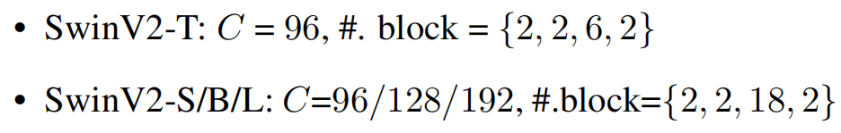
其中 $C$ 是第一个stage的通道数。

作者又进一步扩大Swin Transformer V2到huge size和giant size，分别有6.58亿和30亿参数：

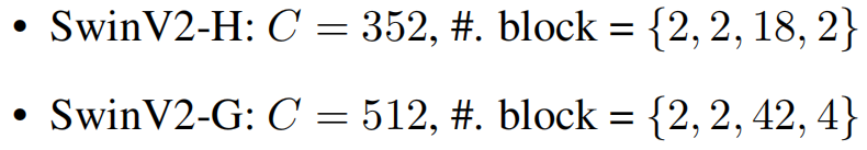
对于SwinV2-H和SwinV2-G，每6层在主分支上额外添加一层layer normalization。

实验结果

表2比较了SwinV2与之前在ImageNet-1K V1和V2上最大/最好的模型。

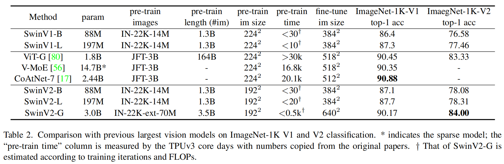
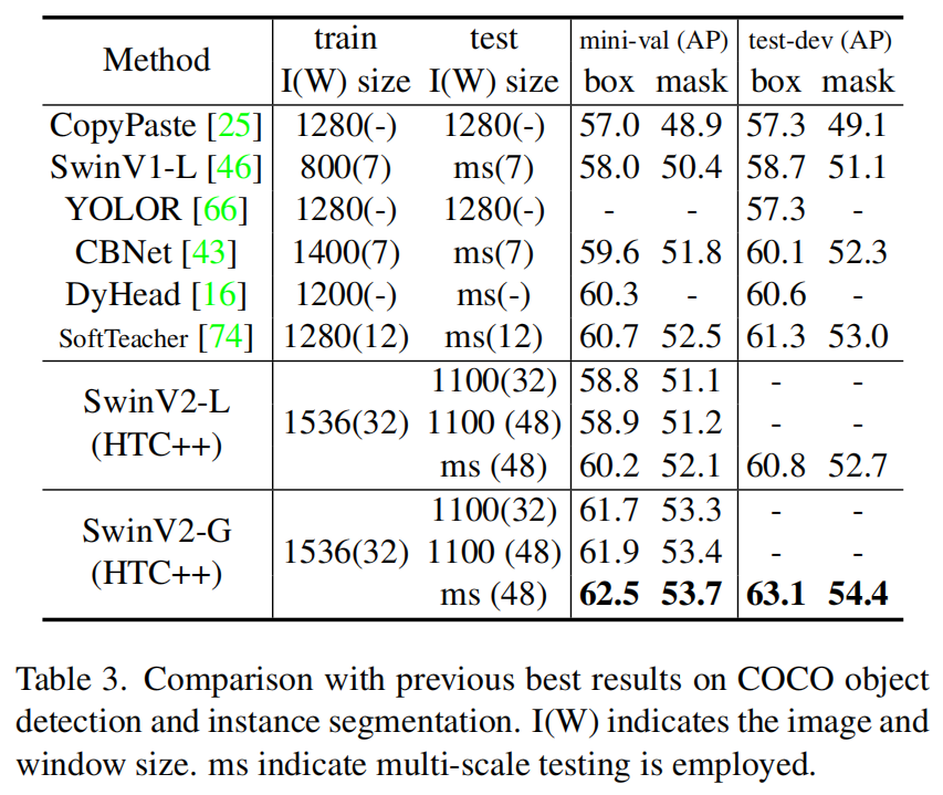
表3是在COCO数据集上之前最好的模型进行对比。

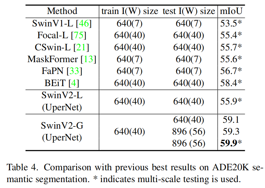
在ADE20K数据集上与之前最好的分割模型的对比结果。

 

代码解析

这里介绍的是timm中的实现。

Post normalization的实现如下，左边是V1，右边是V2，可以看到V2将norm层放到的attention和mlp之后。

Scaled cosine attention的实现如下，cosine similarity的公式是 $\frac{A\cdot B}{\left \| A \right \| \left \| B \right \| }$，分母是 $L2$ 范数，而F.normalize()默认就是 $L2$ 范数。

attn = (F.normalize(q, dim=-1) @ F.normalize(k, dim=-1).transpose(-2, -1))
logit_scale = torch.clamp(self.logit_scale, max=math.log(1. / 0.01)).exp()
attn = attn * logit_scale

在v1中，一共有两张表，一个是relative_position_index，shape=(49, 49)，因为window size=7x7，这里存的是窗口内每个像素点与其它所有像素点之间的相对位置。另一张表是relative_position_bias_table，shape=(169, 3)，其中169=13x13，13=2x7-1，表示窗口内沿一个方向共有13种相对位置关系，3是head的数量。表index在训练过程中为常量，bias的内容是模型优化学习到的，在计算attention时根据index从bias中取值并与attention相加，将位置信息添加到注意力中。

在v2中，下面这段代码是计算index表的，和v1中的函数get_relative_position_index是一模一样的。

# get pair-wise relative position index for each token inside the window
coords_h = torch.arange(self.window_size[0])
coords_w = torch.arange(self.window_size[1])
coords = torch.stack(ndgrid(coords_h, coords_w))  # 2, Wh, Ww
coords_flatten = torch.flatten(coords, 1)  # 2, Wh*Ww
relative_coords = coords_flatten[:, :, None] - coords_flatten[:, None, :]  # 2, Wh*Ww, Wh*Ww
relative_coords = relative_coords.permute(1, 2, 0).contiguous()  # Wh*Ww, Wh*Ww, 2
relative_coords[:, :, 0] += self.window_size[0] - 1  # shift to start from 0
relative_coords[:, :, 1] += self.window_size[1] - 1
relative_coords[:, :, 0] *= 2 * self.window_size[1] - 1
relative_position_index = relative_coords.sum(-1)  # Wh*Ww, Wh*Ww
self.register_buffer("relative_position_index", relative_position_index, persistent=False)

Log-spaced coordinates的实现如下，对应文中的式(4)，将linear-scaled坐标转换成log-scaled坐标。

# get relative_coords_table
relative_coords_h = torch.arange(-(self.window_size[0] - 1), self.window_size[0]).to(torch.float32)  # (15)
relative_coords_w = torch.arange(-(self.window_size[1] - 1), self.window_size[1]).to(torch.float32)  # (15)
relative_coords_table = torch.stack(ndgrid(relative_coords_h, relative_coords_w))  # (2,15,15)
relative_coords_table = relative_coords_table.permute(1, 2, 0).contiguous().unsqueeze(0)  # 1, 2*Wh-1, 2*Ww-1, 2, (1,15,15,2)
if pretrained_window_size[0] > 0:
    relative_coords_table[:, :, :, 0] /= (pretrained_window_size[0] - 1)
    relative_coords_table[:, :, :, 1] /= (pretrained_window_size[1] - 1)
else:
    relative_coords_table[:, :, :, 0] /= (self.window_size[0] - 1)  # 归一化到[-1, 1], 闭区间两侧能取到
    relative_coords_table[:, :, :, 1] /= (self.window_size[1] - 1)
relative_coords_table *= 8  # normalize to -8, 8
relative_coords_table = torch.sign(relative_coords_table) * torch.log2(
    torch.abs(relative_coords_table) + 1.0) / math.log2(8)
 
self.register_buffer("relative_coords_table", relative_coords_table, persistent=False)

Continuous relative position bias的实现如下，对应文中的式(3)，在v1中bias_table是通过网络学习得到的，这里是对coords_table用了一个两层的MLP，其中MLP的参数是通过学习得到的。

# mlp to generate continuous relative position bias
self.cpb_mlp = nn.Sequential(
    nn.Linear(2, 512, bias=True),
    nn.ReLU(inplace=True),
    nn.Linear(512, num_heads, bias=False)
)
 
relative_position_bias_table = self.cpb_mlp(self.relative_coords_table).view(-1, self.num_heads)  # (1,15,15,2)->(1,15,15,3)->(225,3)

最后通过position_index从bias_table中取出对应的bias，和v1中是一样的。

relative_position_bias = relative_position_bias_table[self.relative_position_index.view(-1)].view(
            self.window_size[0] * self.window_size[1], self.window_size[0] * self.window_size[1], -1)  # Wh*Ww,Wh*Ww,nH

最后还有这一步，这一步原文没有提到，希望有理解的大神可以在评论里解释一下。

relative_position_bias = 16 * torch.sigmoid(relative_position_bias)