喵喵爱编程

这个屌丝很懒，什么也没留下！

热门标签

（13-3-02）服装推荐系统：数据集处理——数据清洗_推荐系统coat数据集

作者：喵喵爱编程 | 2024-07-05 05:18:10

踩

推荐系统coat数据集

12.5.2 数据清洗

在经过前面的初步分析之后，可能会发现数据集中存在噪声、缺失值、异常值等问题。为了确保数据的质量和一致性，你需要进行数据清洗。编写文件data_cleaning.ipynb实现数据清洗功能，具体实现流程如下所示。

（1）加载数据集文件，使用给定的文件路径配置信息构建完整的文件路径，以便后续对相应文件进行读取和处理操作。对应的实现代码如下所示：


categorical_column = lambda x: ('NONE' if pd.isna(x) or len(x) == 0 else 'NONE' if x =='None' else x)
 
df_customer = pd.read_csv(CUSTOMER_MASTER_TABLE,
                          converters = 
                                      {                                      
                                       'fashion_news_frequency': categorical_column   
                                      },
                          usecols = ['customer_id', 'FN', 'Active', 'club_member_status','fashion_news_frequency', 'age'],
                          dtype = 
                                  {
                                    'club_member_status': 'category'                                   
                                  }                          
                         )
 
 
df_customer.FN.fillna(0, inplace = True)
df_customer.FN = df_customer.FN.astype(bool)
 
df_customer.Active.fillna(0, inplace = True)
df_customer.Active = df_customer.Active.astype(bool)
 
df_customer.rename(columns = {'FN':'subscribe_fashion_newsletter','Active':'active'}, inplace = True)
df_customer['fashion_news_frequency'] = df_customer['fashion_news_frequency'].astype('category')
 
df_customer.customer_id = df_customer.customer_id.apply(lambda x: int(x[-16:],16) ).astype('int64')
df_customer.head()

（2）读取名为CUSTOMER_MASTER_TABLE的CSV文件，并将特定列进行数据类型转换、重命名和填充缺失值。最后，打印输出df_customer的前几行数据。对应的实现代码如下所示：


categorical_column = lambda x: ('NONE' if pd.isna(x) or len(x) == 0 else 'NONE' if x =='None' else x)
 
df_customer = pd.read_csv(CUSTOMER_MASTER_TABLE,
                          converters =
                                      {                                      
                                       'fashion_news_frequency': categorical_column   
                                      },
 
                         usecols = ['customer_id', 'FN', 'Active', 'club_member_status','fashion_news_frequency', 'age'],
                          dtype =
                                  {
 
                                    'club_member_status': 'category'                                   
                                  }                          
                         )
 
 
df_customer.FN.fillna(0, inplace = True)
df_customer.FN = df_customer.FN.astype(bool)
 
 
df_customer.Active.fillna(0, inplace = True)
df_customer.Active = df_customer.Active.astype(bool)
 
 
df_customer.rename(columns = {'FN':'subscribe_fashion_newsletter','Active':'active'}, inplace = True)
 
df_customer['fashion_news_frequency'] = df_customer['fashion_news_frequency'].astype('category')
 
df_customer.customer_id = df_customer.customer_id.apply(lambda x: int(x[-16:],16) ).astype('int64')
df_customer.head()

执行后输出：


customer_id subscribe_fashion_newsletter active club_member_status fashion_news_frequency age
0 6883939031699146327 False False ACTIVE NONE 49.0
1 -7200416642310594310 False False ACTIVE NONE 25.0
2 -6846340800584936 False False ACTIVE NONE 24.0
3 -94071612138601410 False False ACTIVE NONE 54.0
4 -283965518499174310 True True ACTIVE Regularly 52.0

（3）对df_customer的age列进行描述性统计分析，并绘制箱线图和直方图。对应的实现代码如下所示：


df_customer.age.describe()
sns.boxplot(x = df_customer.age)
sns.displot(df_customer, x = "age",  binwidth = 5)
plt.show()

执行后会显示绘制的箱线图和直方图，如图12-3所示。

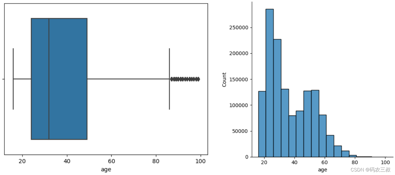
图12-3 绘制的箱线图和直方图

（4）接下来开始移除异常值，通过如下代码计算年龄数据的四分位数(Q1, Q3)和四分位距(IQR)，然后根据上限（upper limit）标记年龄超过上限的客户为异常值。同时，计算年龄的中位数，并将缺失值填充为中位数，并将年龄数据转换为无符号8位整数类型。最后，将生成的数据框的前几行打印出来。


Q1, Q3 = np.nanpercentile(df_customer.age, [25, 75]) 
 
print('Q1 25 percentile of the given data is, ', Q1)
print('Q1 75 percentile of the given data is, ', Q3)
  
IQR = Q3 - Q1 
print('Interquartile range is', IQR)
up_lim = Q3 + 1.5 * IQR
print('Upper limit is', up_lim)
 
df_customer['is_outlier'] = df_customer.age > up_lim
 
age_median = df_customer.age.median(skipna = True)
print(f'Median age: {age_median}')
df_customer.age = df_customer.age.fillna(value = age_median)
df_customer.age = np.uint8(df_customer.age)
 
df_customer.head()

执行后输出：


	customer_id	subscribe_fashion_newsletter	active	club_member_status	fashion_news_frequency	age	is_outlier
0	6883939031699146327	False	False	ACTIVE	NONE	49	False
1	-7200416642310594310	False	False	ACTIVE	NONE	25	False
2	-6846340800584936	False	False	ACTIVE	NONE	24	False
3	-94071612138601410	False	False	ACTIVE	NONE	54	False
4	-283965518499174310	True	True	ACTIVE	Regularly	52	False

（5）接下来开始处理交易数据，首先从pickle文件中读取交易数据到DataFrame，然后对日期时间列进行格式转换，然后进行数据类型转换和列重命名，以减少内存使用和提高数据的可读性。对应的实现代码如下所示：


df_transaction = pd.read_pickle(TRANSACTION_DATA, 
                                compression = 'gzip'                                  
                               )
 
df_transaction.t_dat = pd.to_datetime(df_transaction.t_dat)
 
df_transaction.article_id = pd.to_numeric(df_transaction.article_id, downcast = 'unsigned')
 
df_transaction.price = df_transaction.price.astype('float16')
 
df_transaction.customer_id = df_transaction.customer_id.apply(lambda x: int(x[-16:],16) ).astype('int64')
 
df_transaction.sales_channel_id =  df_transaction.sales_channel_id.apply(lambda x: False if (x == 1) else True)
df_transaction.rename(columns = {'sales_channel_id':'online_sale'}, inplace = True)
 
print("Shape of transaction records:" + str(df_transaction.shape))
 
df_transaction.head()

执行后会输出：


t_dat customer_id article_id price online_sale
0 2018-09-20 -6846340800584936 663713001 0.050842 True
1 2018-09-20 -6846340800584936 541518023 0.030487 True
2 2018-09-20 -8334631767138808638 505221004 0.015236 True
3 2018-09-20 -8334631767138808638 685687003 0.016937 True
4 2018-09-20 -8334631767138808638 685687004 0.016937 True

（6）编写如下所示的代码，首先从交易数据中删除重复记录，并保留第一条记录。然后打印删除重复记录后的交易数据形状，并对交易数据按照"customer_id"和"article_id"进行分组，并统计每个组中"price"的计数。最后使用lambda函数筛选出计数大于1的组，并重新命名计数列为"count"，并将结果重置为新的DataFrame。


df_transaction.drop_duplicates(keep = 'first', inplace = True)
print("Shape of transaction records after droping duplicate:" + str(df_transaction.shape))
df_group = df_transaction.groupby(['customer_id','article_id'])['price'].count().pipe(lambda  dfx: dfx.loc[dfx > 1]).reset_index(name = 'count')
df_group.head()

执行后会输出：


       customer_id	     article_id   count
0	-9223352921020755230	706016001	2
1	-9223343869995384291	519583013	2
2	-9223343869995384291	583534014	3
3	-9223343869995384291	649671009	2
4	-9223343869995384291	655784014	2

（7）编写如下所示的代码，在交易数据中添加一个新的列"index_col"，该列的值为数据的索引。然后将"df_group" DataFrame中的"customer_id"和"article_id"列与"df_transaction" DataFrame进行内连接（inner join）操作，根据这两列进行数据的合并。最后返回合并后的DataFrame的前几行数据。


df_transaction['index_col'] = df_transaction.index
df_group = (df_group[['customer_id','article_id']]
            .merge(df_transaction,           
                    on = ['customer_id','article_id'], 
                    how = 'inner')
            )
df_group.head()

执行后会输出：


customer_id	article_id	  t_dat	price	   online_sale  index_col
0	-9223352921020755230	706016001	2019-10-12	0.033875	False	17854648
1	-9223352921020755230	706016001	2019-10-26	0.033875	False	18327866
2	-9223343869995384291	519583013	2019-03-16	0.010155	True	7428712
3	-9223343869995384291	519583013	2019-03-20	0.010155	True	7584492
4	-9223343869995384291	583534014	2019-02-21	0.014389	True	6435020

（8）编写如下代码对DataFrame按照"t_dat"列进行排序，然后计算每个购买记录的上一次购买时间，并添加到DataFrame中。最后计算每个购买记录与上一次购买时间之间的时间间隔，并将结果添加到DataFrame中。


df_group.sort_values(by = 't_dat',  inplace = True)
df_group['previous_purchase'] = df_group.groupby(['customer_id','article_id'])['t_dat'].shift(periods = 1)
df_group['previous_purchase'] = pd.to_datetime(df_group['previous_purchase'], errors = 'coerce')
df_group['time_pass_before_last_purchase'] = ((df_group['t_dat'] - df_group['previous_purchase']).dt.days).fillna(0).astype(int)
df_group.head()

执行后会输出：


	customer_id	article_id	t_dat	price	online_sale	index_col	previous_purchase	time_pass_before_last_purchase
1845563	2818613237059253259	562245058	2018-09-20	0.033875	False	2103	NaT	0
39824	-8971660418312476665	571436010	2018-09-20	0.012184	False	3697	NaT	0
39825	-8971660418312476665	571436010	2018-09-20	0.013542	False	3698	2018-09-20	0
1667034	1648773112888926075	651327001	2018-09-20	0.018677	True	544	NaT	0
2740283	8630231611017253359	700833004	2018-09-20	0.064392	True	14252	NaT	0

（9）绘制顾客在最后一次购买之前经过的天数的直方图，对应的实现代码如下所示：


usecol = ['article_id','product_type_name']
df_articles = pd.read_csv(ARTICLES_MASTER_TABLE, 
                          usecols = usecol
                         )
 
df_subset = df_group[df_group.time_pass_before_last_purchase != 0]
df_subset = df_articles.merge(df_subset,
                              on = 'article_id', 
                              how ='inner')
df_subset.head()
 
del [df_articles]
gc.collect()
                              
 
plt.figure(figsize = (15,5), 
           dpi = 100, 
           clear = True,
           constrained_layout =  True
           )
 
ax = sns.histplot(data = df_subset, x = 'time_pass_before_last_purchase', bins = 74)
 
ax.set_xticks(list(range(0,740,10)))
ax.set_xlim(0,370)
ax.set_xlabel("Days elapsed before last purchase")
ax.set_ylabel("Count")
plt.show()

首先，从"ARTICLES_MASTER_TABLE"中读取"article_id"和"product_type_name"两列的数据，存储在DataFrame "df_articles"中。
从"df_group"中筛选出"time_pass_before_last_purchase"不等于0的记录，存储在DataFrame "df_subset"中。
将"df_articles"和"df_subset"根据"article_id"列进行内连接，得到新的DataFrame "df_subset"。
绘制直方图，展示"time_pass_before_last_purchase"的分布情况。
对内存中的变量进行删除和垃圾回收操作。
最后，显示绘制的直方图。

绘制的直方图效果如图12-4所示。

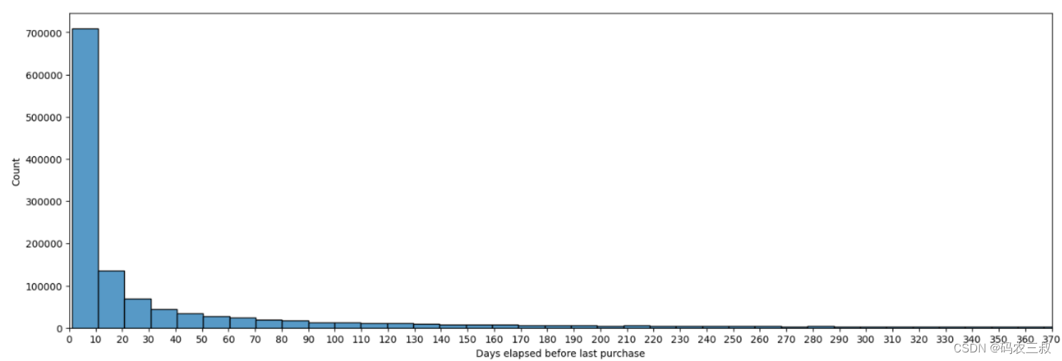
图12-4 顾客在最后一次购买之前经过的天数的直方图

（10）通过如下代码绘制产品类型的计数柱状图，首先创建一个图形对象（Figure）并设置其属性，然后使用Seaborn库的countplot函数绘制柱状图，其中X轴表示产品类型，Y轴表示计数。通过设置旋转角度使X轴标签垂直显示。最后，显示绘制的图形并清除图形对象以释放资源。


fig_WS = plt.figure(num = 1, 
                    figsize = (15,5), 
                    dpi = 100, 
                    clear = True,
                    constrained_layout =  True
                    )
 
ax = sns.countplot(data = df_subset, 
                   x = 'product_type_name',
                   order = df_subset['product_type_name'].value_counts().index
                   )
 
ax.set_xticklabels(ax.get_xticklabels(), 
                   rotation = 90                   
                   )
 
ax.set_xlabel("Product Type")
ax.set_ylabel("Count")
 
plt.show()
fig_WS.clf()

执行后会绘制产品类型的计数柱状图，如图12-5所示。

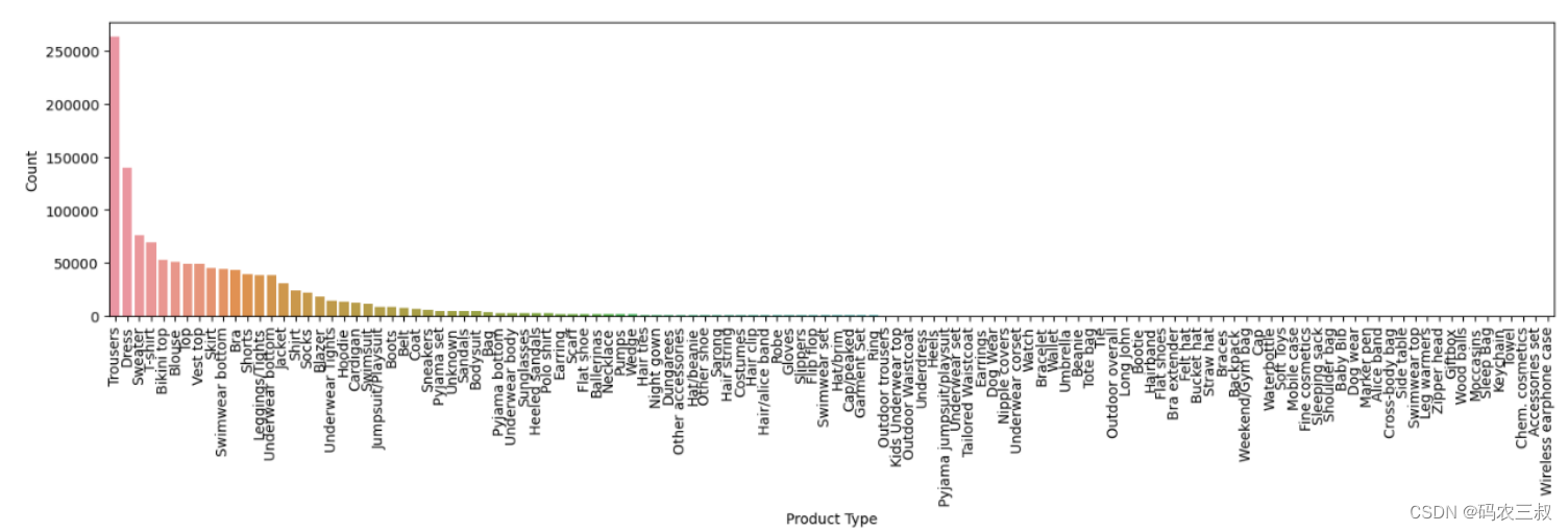
图12-5 产品类型的计数柱状图

在众多商品中，属于配件类别的物品，例如内衣、帽子、发夹、钱包、腰带等，用户可能会多次购买。几乎85%的服装重新购买的物品属于服装类别，如裤子、连衣裙、毛衣、T恤等。很可能用户不会购买相同的物品多次，因为不同颜色的物品会有不同的article_id。几乎90%的重新购买的物品在30天内完成，而H&M有30天的退货政策。因此，我们可以假设这些是退货的物品，用户以不同尺码购买了相同的物品，而H&M将其视为新交易，并可能在维护一个单独的退货交易表。

由于我们希望向用户推荐与他们过去购买的物品类似的新物品，所以我们可以删除这些重复的物品，其中他们再次购买了相同的物品，只保留用户对该物品最后一次交易的记录。

（11）首先通过如下代码对数据框（DataFrame）进行排序，按照customer_id、article_id和t_dat进行降序排序。这样做的目的是删除重复的购买记录，并保留每个顾客对每个物品的第一次购买记录。


df_group.sort_values(by = ['customer_id','article_id','t_dat'], inplace = True, ascending = False)
df_group.head()

执行后会输出:


	customer_id	article_id	t_dat	price	online_sale	index_col	previous_purchase	time_pass_before_last_purchase
2831516	9223333063893176977	607834005	2018-11-18	0.017776	False	2620551	2018-11-08	10
2831515	9223333063893176977	607834005	2018-11-08	0.025406	True	2265236	NaT	0
2831514	9223148401910457466	830770001	2019-12-14	0.029358	False	20126479	2019-11-08	36
2831513	9223148401910457466	830770001	2019-11-08	0.033875	False	18773300	NaT	0
2831512	9223148401910457466	767377003	2019-06-09	0.050842	False	11590886	2019-06-06	3

（12）编写如下代码，从主交易数据表中删除所有重复的行。从df_group数据表中删除重复的顾客和物品组合，只保留每个组合的第一次购买记录。选择特定的列（article_id、t_dat、customer_id、price、online_sale）从df_group数据表中提取出来。将提取的数据表与主交易数据表进行连接，添加到主交易数据表的末尾。然后，从主交易数据表中删除列"index_col"。最后，显示更新后的主交易数据表的前几行。


df_transaction.drop(index = df_group.index_col, inplace = True)
df_group.drop_duplicates(subset = ['customer_id','article_id'], keep = 'first', inplace = True)
usecol = ['article_id', 't_dat', 'customer_id', 'price', 'online_sale'] 
df_transaction = pd.concat([df_transaction, 
                           df_group[usecol]
                           ], 
                           axis = 0)                    
df_transaction.drop(columns = ['index_col'], 
                    axis = 1, 
                    inplace = True)
df_transaction.head()

执行后会输出：


t_dat customer_id article_id price online_sale
1 2018-09-20 -6846340800584936 541518023 0.030487 True
2 2018-09-20 -8334631767138808638 505221004 0.015236 True
3 2018-09-20 -8334631767138808638 685687003 0.016937 True
4 2018-09-20 -8334631767138808638 685687004 0.016937 True
5 2018-09-20 -8334631767138808638 685687001 0.016937 True

（13）接下来开始删除异常值记录，为什么要这样做呢？因为每种商品都是不同的，售价也不同。因此，不能简单地对定价列应用异常值处理，而不考虑每种商品的价格。我们将按商品分组，找出该商品组类型中价格的异常值。

注意：由于动态定价的存在，某些商品的价格可能比其他商品高得多。

编写如下代码绘制在线销售与离线销售价格散点图，首先将数据中在线销售和离线销售的价格分别提取出来，然后进行描述性统计分析。接下来，打印在线销售价格的描述统计信息和离线销售价格的描述统计信息。然后创建一个图表，并将在线销售和离线销售的价格分别以散点图的形式绘制出来。最后，设置图表的标题、坐标轴标签和刻度，并显示绘制的图表。


online_sales = df_transaction[df_transaction.online_sale == 1]['price']
offline_sales = df_transaction[df_transaction.online_sale == 0]['price']
 
print("="*20 + "Online Sales" + "="*20)
print(online_sales.describe())
 
print("="*20 + "Offline Sales" + "="*20)
print(offline_sales.describe())
fig = plt.figure(figsize = (15,10))
 
y_index = range(online_sales.shape[0])
ax = sns.scatterplot(y = online_sales, x = y_index, color = ['red'], label = "Online")
 
y_index = range(offline_sales.shape[0])
ax = sns.scatterplot(y = offline_sales, x = y_index, color = ['blue'] , label = "Offline")
 
ax.set_title("Sales Price")
ax.set_ylabel("Price")
ax.set_xlabel("Index")
ax.set_yticks(np.linspace(0.01, 0.5, num = 40))
#ax.grid()
ax.legend(title = 'Sales Channel')
 
plt.show()

执行效果如图12-6所示。

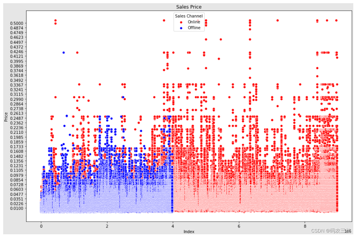
图12-6 在线销售与离线销售价格散点图

（14）编写如下代码，使用散点图绘制在线销售和离线销售的价格分布情况。


fig = plt.figure(figsize = (15,10))
 
#online_sales = df_transaction[df_transaction.online_sale == 1]['price'].values
sorted_online_price = np.sort(online_sales)[::-1]
y_index = range(online_sales.shape[0])
ax = sns.scatterplot(y = sorted_online_price, x = y_index, color = ['red'], label = "Online")
 
 
#offline_sales = df_transaction[df_transaction.online_sale == 0]['price'].values
sorted_offline_price = np.sort(offline_sales)[::-1]
y_index = range(offline_sales.shape[0])
ax = sns.scatterplot(y = sorted_offline_price, x = y_index, color = ['blue'] , label = "Offline")
 
ax.set_title("Sorted Sales Price")
ax.set_ylabel("Price")
ax.set_xlabel("Index")
ax.set_yticks(np.linspace(0.01, 0.5, num = 50))
ax.grid()
ax.legend(title = 'Sales Channel')
 
plt.show()

执行效果如图12-7所示。

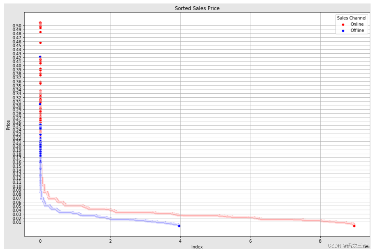
图12-7 在线销售和离线销售的价格分布情况散点图

（15）请看下面的两段代码，其中第1段代码用于统计价格在区间[0.01, 0.17]内的数据所占的比例，并输出结果。第2段代码用于统计价格大于0.17的数据所占的比例，并输出结果。


per = df_transaction[(df_transaction.price >=0.01) & (df_transaction.price<=0.17)].shape[0]
per = per/df_transaction.shape[0]
print(f'Percentage of data between [0.01, 0.17]: {per}')
per = df_transaction[(df_transaction.price > 0.17)].shape[0]
per = per/df_transaction.shape[0]
print(f'Percentage of data more then 0.17: {per}')
 
fig, axis = plt.subplots(nrows = 1, ncols = 2, figsize = (20,10))
sns.distplot(online_sales, ax = axis[0])
sns.distplot(offline_sales, ax = axis[1])
plt.suptitle("Distribution of the sale price")
axis[0].set_title("Online Sale Price")
axis[1].set_title("Offline Sale Price")
plt.show()

执行后会创建一个大小为20x10的图形，并分为1行2列的子图。左侧子图显示在线销售价格的分布情况，右侧子图显示离线销售价格的分布情况。图形的标题为"Distribution of the sale price"，左侧子图标题为"Online Sale Price"，右侧子图标题为"Offline Sale Price"。如图12-8所示。

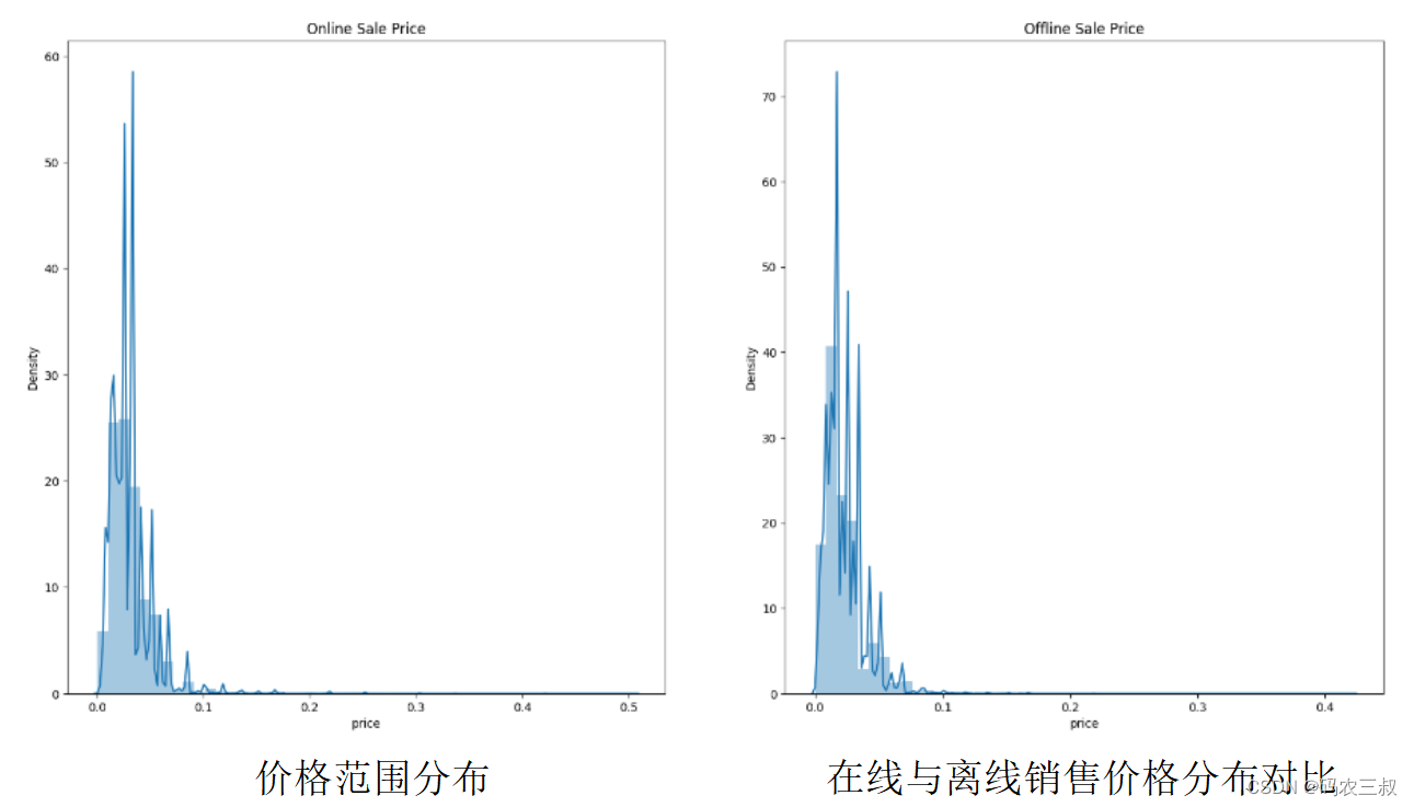
图12-8 执行效果

（16）对相似的product_type_name进行分组，为了减少唯一product type name的基数，采取以下步骤实现：

创建一个新的列"product_type_name_org"，复制原始值并更新"product_type_name"。
根据它们所属的类别对产品进行分组。

对应的实现代码如下所示：


unique_product_type = df_article.product_type_name.unique()
print(f'Number of unique product type before: {len(unique_product_type)}')
 
colname = 'product_type_name_org'
colindex = ['product_type_name']
# 将原始值复制到新列“_org”
df_article[colname] = df_article.product_type_name
 
# 合并所有“hat”，“cap”，“beanie”产品类型为“Hat Cap”
# Beanie看起来像某种帽子
filters = ["Hat", "Cap", "Beanie"]
items = hlpeda.filter_types(filters, unique_product_type)
rowindex = df_article[df_article.product_type_name.isin(items)].index.tolist()
df_article.loc[rowindex, colindex] = "Hat Cap"
 
# 将所有“Wood balls”，“Side table”等产品类型合并为“Cloths Care”
filters = ["Wood balls", "Side table", "Stain remover spray", "Sewing kit", "Clothing mist", "Zipper head"]
items = hlpeda.filter_types(filters, unique_product_type)
rowindex = df_article[df_article.product_type_name.isin(items)].index.tolist()
df_article.loc[rowindex, colindex] = "Cloths Care"
 
# 将所有“Ring”，“Necklace”，“Bracelet”，“Earring”产品类型合并为“Jewellery”
filters = ["Ring", "Necklace", "Bracelet", "Earring"]
items = hlpeda.filter_types(filters, unique_product_type)
rowindex = df_article[df_article.product_type_name.isin(items)].index.tolist()
df_article.loc[rowindex, colindex] = "Jewellery"
 
# 将所有“Polo shirt”产品类型合并为“Shirt”
filters = ["Polo shirt"]
items = hlpeda.filter_types(filters, unique_product_type)
rowindex = df_article[df_article.product_type_name.isin(items)].index.tolist()
df_article.loc[rowindex, colindex] = "Shirt"
 
# 将所有“Bag”产品类型合并为“Bag”
filters = ["Bag", 'Backpack']
items = hlpeda.filter_types(filters, unique_product_type)
rowindex = df_article[df_article.product_type_name.isin(items)].index.tolist()
df_article.loc[rowindex, colindex] = "Bag"
 
# 将所有“Swimwear bottom”，“Swimsuit”，“Bikini top”产品类型合并为“Swimwear”
filters = ["Swimwear"]
items = hlpeda.filter_types(filters, unique_product_type)
rowindex = df_article[df_article.product_type_name.isin(items)].index.tolist()
df_article.loc[rowindex, colindex] = "Swimwear"
 
# 将所有“Underwear bottom”，“Underwear Tights”，“Underwear body”，“Long John”产品类型合并为“Underwear”
filters = ["Underwear", "Long John"]
items = hlpeda.filter_types(filters, unique_product_type)
rowindex = df_article[df_article.product_type_name.isin(items)].index.tolist()
df_article.loc[rowindex, colindex] = "Underwear"
 
# 将所有“Hair”，“Alice band”，“Hairband”产品类型合并为“Hair Accessories”
filters = ["Hair", "Alice band", "Hairband"]
items = hlpeda.filter_types(filters, unique_product_type)
rowindex = df_article[df_article.product_type_name.isin(items)].index.tolist()
df_article.loc[rowindex, colindex] = "Hair Accessories"
 
# 将所有“Sandals”，“Heeled sandals”，“Wedge”，“Pumps”，“Slippers”产品类型合并为“Sandals”
# Ballerinas是一种用于芭蕾舞演出的凉鞋类型
filters = ["Sandals", "Heels", "Flip flop", "Wedge", "Pump", "Slipper", "Ballerinas"]
items = hlpeda.filter_types(filters, unique_product_type)
rowindex = df_article[df_article.product_type_name.isin(items)].index.tolist()
df_article.loc[rowindex, colindex] = "Sandals"
 
# 将所有“Toy”，“Soft Toys”产品类型合并为“Toys”
filters = ["Toy"]
items = hlpeda.filter_types(filters, unique_product_type)
rowindex = df_article[df_article.product_type_name.isin(items)].index.tolist()
df_article.loc[rowindex, colindex] = "Toy"
 
# 将所有“Flat Shoe”，“Other Shoe”，“Boots”，“Sneakers”产品类型合并为“Shoe”
filters = ["shoe", "Boot", "Leg warmer", "Sneakers"]
items = hlpeda.filter_types(filters, unique_product_type)
rowindex = df_article[df_article.product_type_name.isin(items)].index.tolist()
df_article.loc[rowindex, colindex] = "Shoe"
 
# 将所有“Dog wear”产品类型合并为“Dog wear”
filters = ["Dog wear"]
items = hlpeda.filter_types(filters, unique_product_type)
rowindex = df_article[df_article.product_type_name.isin(items)].index.tolist()
df_article.loc[rowindex, colindex] = "Dog wear"
 
# 将所有“Sunglasses”，“EyeGlasses”产品类型合并为“Glasses”
filters = ["glasses"]
items = hlpeda.filter_types(filters, unique_product_type)
rowindex = df_article[df_article.product_type_name.isin(items)].index.tolist()
df_article.loc[rowindex, colindex] = "Glasses"
 
# 将所有“Cosmetics”，“Chem. Cosmetics”产品类型合并为“Cosmetics”
filters = ["Cosmetics"]
items = hlpeda.filter_types(filters, unique_product_type)
rowindex = df_article[df_article.product_type_name.isin(items)].index.tolist()
df_article.loc[rowindex, colindex] = "Cosmetics"
 
# 将所有“earphone case”，“case”产品类型合并为“Mobile Accesories”
filters = ["earphone case", "case"]
items = hlpeda.filter_types(filters, unique_product_type)
rowindex = df_article[df_article.product_type_name.isin(items)].index.tolist()
df_article.loc[rowindex, colindex] = "Mobile Accesories"
 
# 将所有“Bra extender”产品类型合并为“Bra”
filters = ["Bra extender"]
items = hlpeda.filter_types(filters, unique_product_type)
rowindex = df_article[df_article.product_type_name.isin(items)].index.tolist()
df_article.loc[rowindex, colindex] = "Bra"
 
# 将所有“Nipple covers”产品类型（不属于Nightwear部门名称）合并为“Bar”
filters = ["Nipple covers"]
rowindex = df_article[(df_article.department_name != 'Nightwear') &
                      (df_article.product_type_name.isin(filters))].index.tolist()
df_article.loc[rowindex, colindex] = "Bra"
 
# 将所有“Tailored Waistcoat”，“Outdoor Waistcoat”产品类型合并为“Waistcoat”
filters = ["Waistcoat"]
items = hlpeda.filter_types(filters, unique_product_type)
rowindex = df_article[df_article.product_type_name.isin(items)].index.tolist()
df_article.loc[rowindex, colindex] = "Waistcoat"
 
# 将“Outdoor trousers”产品类型合并为“Trousers”
filters = ["Outdoor trousers"]
items = hlpeda.filter_types(filters, unique_product_type)
rowindex = df_article[df_article.product_type_name.isin(items)].index.tolist()
df_article.loc[rowindex, colindex] = "Trousers"
 
# UnderDress是与某些裙子一起穿的。
# 因此，让我们将它们与Dress部分分组，因为如果用户以前购买了裙子，他们可能需要搭配着穿的UnderDress
filters = ["Underdress"]
items = hlpeda.filter_types(filters, unique_product_type)
rowindex = df_article[df_article.product_type_name.isin(items)].index.tolist()
df_article.loc[rowindex, colindex] = "Dress"
 
# 将“Towel”，“Blanket”，“Cushion”，“Waterbottle”，“Robe”产品类型合并为“House Accesories”
filters = ["Towel", "Blanket", "Cushion", "Waterbottle", "Robe"]
items = hlpeda.filter_types(filters, unique_product_type)
rowindex = df_article[df_article.product_type_name.isin(items)].index.tolist()
df_article.loc[rowindex, colindex] = "House Accesories"
 
print(f'Number of new unique product type after: {df_article.product_type_name.nunique()}')

执行后会输出显示数据框中的新唯一产品类型的数量：


Number of unique product type before: 130
 
Number of new unique product type after: 66

（17）绘制一个水平条形图，显示每个产品类型的数量统计。对应的实现代码如下所示：


class_label_cnt = df_article.product_type_name.value_counts()
fig = plt.figure(figsize = (10,20))
class_label_cnt.plot.barh()

执行效果如图12-9所示。

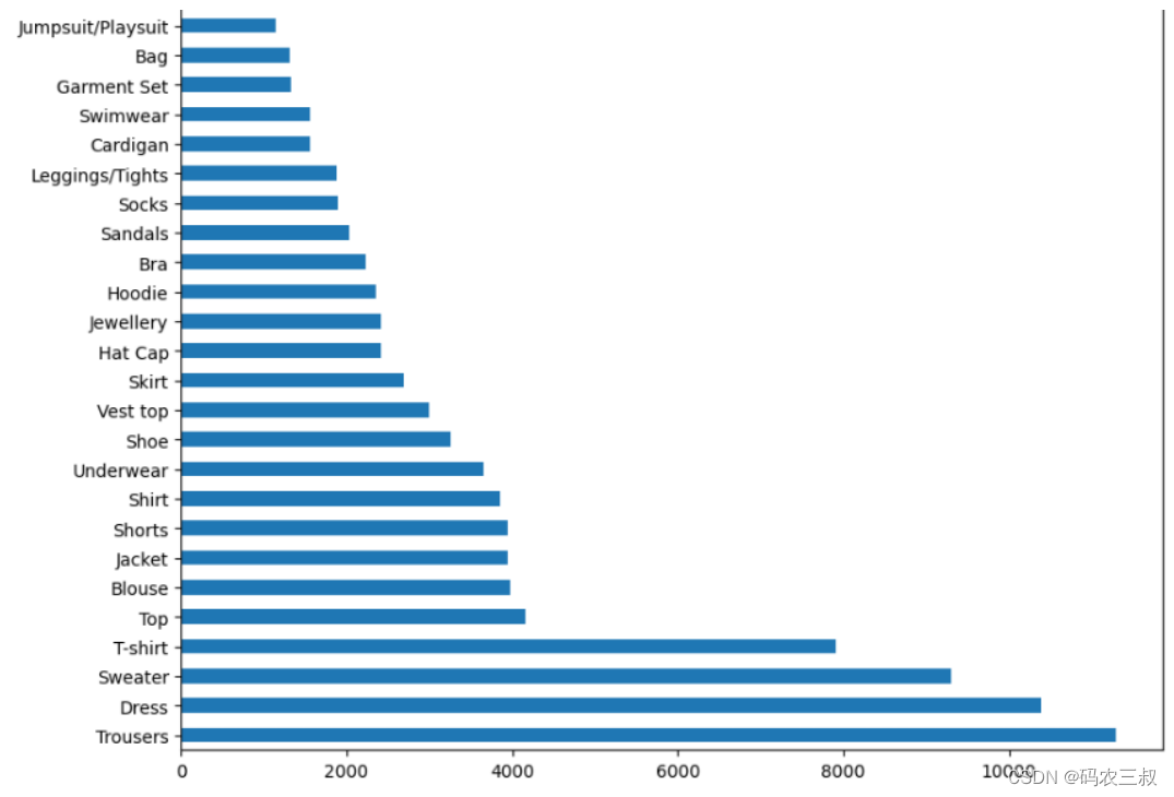
图12-9 产品类型数量统计条形图

注意：探索性数据分析和特征工程

在数据清洗之后，你可以进行更深入的探索性数据分析（EDA）和特征工程。EDA可以帮助你理解数据集中的关系、趋势和分布，为后续的建模和预测准备好数据。特征工程则涉及从原始数据中提取、转换和创建新特征，以便用于机器学习模型的训练。编写文件eda_feature_eng.ipynb实现探索性数据分析和特征工程功能，为节省本书篇幅，将不再讲解这个文件的具体实现过程。

未完待续

声明：本文内容由网友自发贡献，不代表【wpsshop博客】立场，版权归原作者所有，本站不承担相应法律责任。如您发现有侵权的内容，请联系我们。转载请注明出处：https://www.wpsshop.cn/w/喵喵爱编程/article/detail/789302