
基于Python+Tkinter GUI 的模式识别水果分类小程序_基于python的水果分级系统
赞
踩
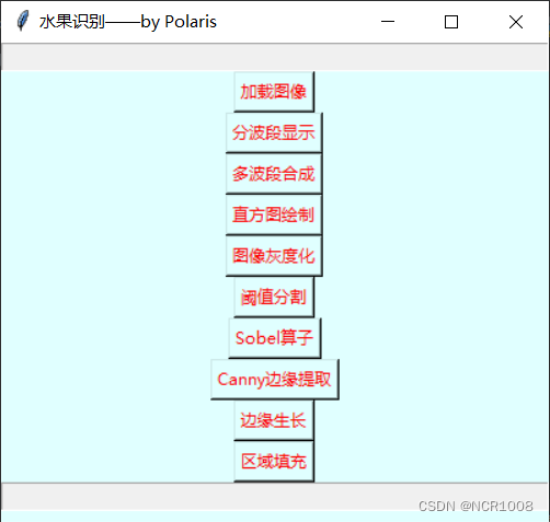
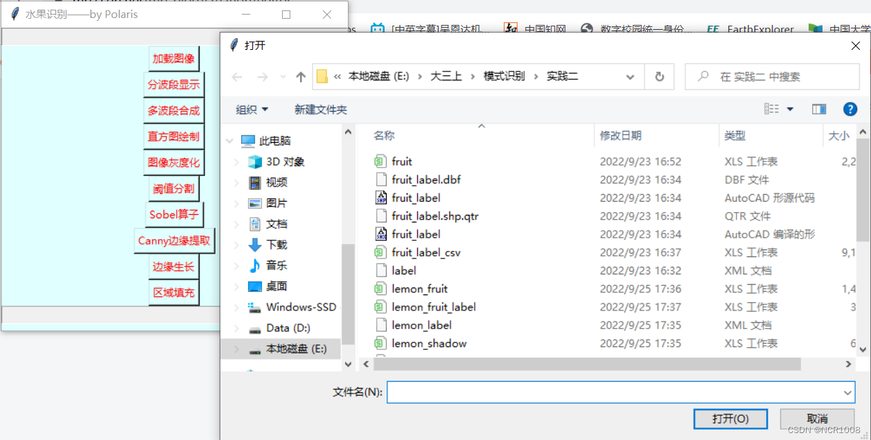
采用Python语言编写,并结合Tkinter GUI工具制作交互式小程序开发,实现了简单的水果的边缘提取和分类。如图1-A,用户可以自定义选择路径并输出,同时可以在对话框中输入/输出结果,如图1-B。
|
|
|
| A 界面展示 | B 交互展示 |
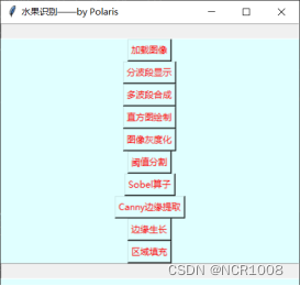
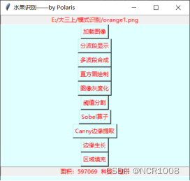
图1 Tkinter GUI 展示
技术路线
本次课程实践一整体设计分为三个部分:
- 利用Python实现图像处理的基础功能
- 利用Python实现图像二值化并提取边缘
- 利用①中的波谱信息以及②中处理后的边缘特征对水果进行分类
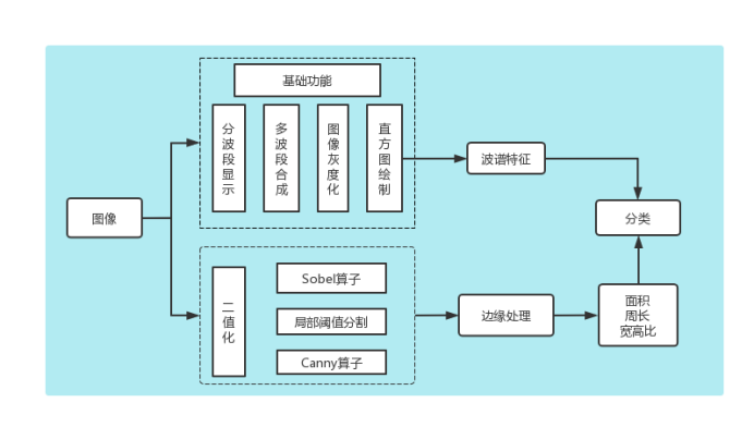
图2 技术路线图
一、界面设计部分
利用python中的tkinter GUI 进行交互式设计
- def __init__(self, master, entry, entry1):
- self.master = master
- self.entry = entry
- self.entry1 = entry1
- # self.gray = gray
- entry = tk.Entry(self.master, state='readonly', text=path, width=100, bg="#E0FFFF", justify='center')
- entry.configure(fg='red', bg="#E0FFFF")
- entry.pack()
- self.b1 = tk.Button(self.master, text='加载图像', command=self.select_img, fg="red", bg="#E0FFFF")
- self.b1.pack()
- self.b2 = tk.Button(self.master, text='分波段显示', command=self.seperateband, fg="red", bg="#E0FFFF")
- self.b2.pack()
- self.b3 = tk.Button(self.master, text='多波段合成', command=self.multibands, fg="red", bg="#E0FFFF")
- self.b3.pack()
- self.b4 = tk.Button(self.master, text='直方图绘制', command=self.historgram, fg="red", bg="#E0FFFF")
- self.b4.pack()
- self.b5 = tk.Button(self.master, text='图像灰度化', command=self.Gray, fg="red", bg="#E0FFFF")
- self.b5.pack()
- self.b6 = tk.Button(self.master, text='阈值分割', command=self.binary, fg="red", bg="#E0FFFF")
- self.b6.pack()
- self.b7 = tk.Button(self.master, text='Sobel算子', command=self.Sobel, fg="red", bg="#E0FFFF")
- self.b7.pack()
- self.b8 = tk.Button(self.master, text='Canny边缘提取', command=self.boundary, fg="red", bg="#E0FFFF")
- self.b8.pack()
- self.b9 = tk.Button(self.master, text='边缘生长', command=self.grow, fg="red", bg="#E0FFFF")
- self.b9.pack()
- self.b10 = tk.Button(self.master, text='区域填充', command=self.fillgrow, fg="red", bg="#E0FFFF")
- self.b10.pack()
- entry1 = tk.Entry(self.master, state='readonly', text=num, width=100, bg="#E0FFFF", justify='center')
- entry1.configure(fg='red', bg="#E0FFFF")
- entry1.pack()
二、图像读取
算法步骤
- Tkinter交互式选择图片
- GDAL库读取影像
- 借助matplotlib显示
-
 源代码
源代码 -
- def select_img(self):
- # 路径选择框
- path_ = tk.filedialog.askopenfilename()
- path.set(path_)
- print('path', path_)
- self.entry = path_
- datafile = gdal.Open(str(path_))
- win1 = tk.Toplevel(self.master)
- win1.title('图像加载')
- win1.geometry('600x400')
- plt.rcParams['font.sans-serif'] = ['SimHei']
- plt.rcParams['axes.unicode_minus'] = False
- fig1 = plt.figure(figsize=(6, 4))
- canvas1 = FigureCanvasTkAgg(fig1, master=win1)
- canvas1.draw()
- canvas1.get_tk_widget().grid()
- band1 = datafile.GetRasterBand(1).ReadAsArray()
- band2 = datafile.GetRasterBand(2).ReadAsArray()
- band3 = datafile.GetRasterBand(3).ReadAsArray()
- img1 = np.dstack((band1, band2, band3))
- ax1 = fig1.add_subplot(111)
- ax1.set_title('真彩色', fontsize=10)
- ax1.imshow(img1)
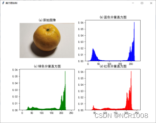
三、直方图绘制
算法步骤
- GDAL逐个读取波段
- 对于每个波段,将[0,255]划分为等间隔的小区间,并统计每个区间上样本出现的频数之和。
- Matplotlib显示
源代码
- def historgram(self):
- win4 = tk.Toplevel(self.master)
- win4.title('直方图绘制')
- win4.geometry('800x600')
- src = gdal.Open(str(self.entry))
- r = src.GetRasterBand(1).ReadAsArray()
- g = src.GetRasterBand(2).ReadAsArray()
- b = src.GetRasterBand(3).ReadAsArray()
- plt.rcParams['font.sans-serif'] = ['SimHei']
- plt.rcParams['axes.unicode_minus'] = False
- fig4 = plt.figure(figsize=(8, 6))
- canvas4 = FigureCanvasTkAgg(fig4, master=win4)
- canvas4.draw()
- canvas4.get_tk_widget().grid()
- # 真彩色
- img = np.dstack([r, g, b])
- ax1 = fig4.add_subplot(221)
- plt.imshow(img)
- plt.axis('off')
- ax1.set_title("(a)原始图像")
-
- # 绘制蓝色分量直方图
- ax2 = fig4.add_subplot(222)
- plt.hist(b.ravel(), bins=256, density=1, facecolor='b', edgecolor='b', alpha=0.75)
- # plt.xlabel("x")
- # plt.ylabel("y")
- ax2.set_title("(b)蓝色分量直方图")
-
- # 绘制绿色分量直方图
- ax3 = fig4.add_subplot(223)
- plt.hist(g.ravel(), bins=256, density=1, facecolor='g', edgecolor='g', alpha=0.75)
- # plt.xlabel("x")
- # plt.ylabel("y")
- ax3.set_title("(c)绿色分量直方图")
-
- # 绘制红色分量直方图
- ax4 = fig4.add_subplot(224)
- plt.hist(r.ravel(), bins=256, density=1, facecolor='r', edgecolor='r', alpha=0.75)
- # plt.xlabel("x")
- # plt.ylabel("y")
- ax4.set_title("(d)红色分量直方图")
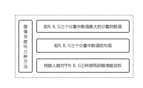
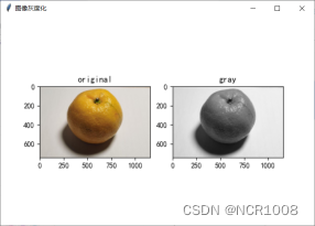
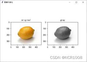
四、图像灰度化
常见的图像灰度化有三种方式:
算法步骤
- GDAL逐波段读取图像
- 选择r、g、b三波段(有些图像为32bit,及包括RGB+Alpha位)
- 将r、g、b三波段利用numpy组合
- 利用rgb2gray函数进行转换,对应转化比例如表三所示
- Matplotlib显示
源代码
- def Gray(self):
- win5 = tk.Toplevel(self.master)
- win5.title('图像灰度化')
- win5.geometry('600x400')
- fig5 = plt.figure(figsize=(6, 4))
- canvas5 = FigureCanvasTkAgg(fig5, master=win5)
- canvas5.draw()
- canvas5.get_tk_widget().grid()
- datafile = gdal.Open(str(self.entry))
- band1 = datafile.GetRasterBand(1).ReadAsArray()
- band2 = datafile.GetRasterBand(2).ReadAsArray()
- band3 = datafile.GetRasterBand(3).ReadAsArray()
- img0 = np.dstack((band1, band2, band3))
- # 读入中文路径
- img = cv2.imdecode(np.fromfile(self.entry, dtype=np.uint8), cv2.IMREAD_COLOR)
- plt.rcParams['font.sans-serif'] = ['SimHei']
- plt.rcParams['axes.unicode_minus'] = False
- ax1 = fig5.add_subplot(121)
- ax1.imshow(img0)
- ax1.set_title('original')
- # 灰度化
- ax2 = fig5.add_subplot(122)
- ax2.set_title('gray')
- gray = cv2.cvtColor(img, cv2.COLOR_RGB2GRAY)
- # gray = rgb2gray(img)
- ax2.imshow(gray, cmap=plt.get_cmap('gray'))
-
- def rgb2gray(rgb):
- # 灰度化原理Y' = 0.299 R + 0.587 G + 0.114 B
- return np.dot(rgb[..., :3], [0.299, 0.587, 0.114])
五、边缘检测
常用的边缘检查的方法大致可以分为两类:①基于查找:通过寻找图像一阶导数中最大值和最小值来检测边界,例如Sobel算子、Roberts Cross算法等。②基于零穿越的:通过寻找图像二阶导数零穿越来寻找边界,例如Canny算子、Laplacian算子等。
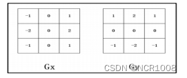
5.1Sobel算子
算法介绍
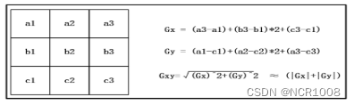
Sobel算子思想:取 3 行 3 列的图像数据,将图像数据与对应位置的算子的值相乘再相加,得到x方向的Gx,和y方向的Gy,将得到的Gx和Gy,平方后相加,再取算术平方根,得到Gxy,近似值为和绝对值之和。将计算得到的阈值比较。若大于阈值,则表明该点为边界点,设置DN值为0,否则为255。
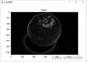
结果
源代码
- def Sobel(self):
- win7 = tk.Toplevel(self.master)
- win7.title('Sobel算子')
- win7.geometry('600x400')
- fig7 = plt.figure(figsize=(6, 4))
- canvas7 = FigureCanvasTkAgg(fig7, master=win7)
- canvas7.draw()
- canvas7.get_tk_widget().grid()
- img = cv2.imdecode(np.fromfile(self.entry, dtype=np.uint8), cv2.IMREAD_COLOR)
- plt.rcParams['font.sans-serif'] = ['SimHei']
- plt.rcParams['axes.unicode_minus'] = False
- # 转灰度图像
- d = cv2.cvtColor(img, cv2.COLOR_RGB2GRAY)
- sp = d.shape
- print(sp)
- height = sp[0]
- weight = sp[1]
- sx = np.array([[-1, 0, 1], [-2, 0, 2], [-1, 0, 1]])
- sy = np.array([[-1, -2, -1], [0, 0, 0], [1, 2, 1]])
- dSobel = np.zeros((height, weight))
- dSobelx = np.zeros((height, weight))
- dSobely = np.zeros((height, weight))
- Gx = np.zeros(d.shape)
- Gy = np.zeros(d.shape)
- for i in range(height - 2):
- for j in range(weight - 2):
- Gx[i + 1, j + 1] = abs(np.sum(d[i:i + 3, j:j + 3] * sx))
- Gy[i + 1, j + 1] = abs(np.sum(d[i:i + 3, j:j + 3] * sy))
- dSobel[i + 1, j + 1] = (Gx[i + 1, j + 1] * Gx[i + 1, j + 1] + Gy[i + 1, j + 1] * Gy[
- i + 1, j + 1]) ** 0.5
- dSobelx[i + 1, j + 1] = np.sqrt(Gx[i + 1, j + 1])
- dSobely[i + 1, j + 1] = np.sqrt(Gy[i + 1, j + 1])
- a = np.uint8(dSobel)
- b = np.uint8(dSobelx)
- c = np.uint8(dSobel)
- img = img[:, :, ::-1]
- image1 = np.dstack([a, a, a])
- image2 = np.dstack([b, b, b])
- image3 = np.dstack([c, c, c])
- ax1 = fig7.add_subplot(111)
- ax1.imshow(image1)
- ax1.set_title('Sobel')
5.2 阈值分割
算法介绍
本问采用采取自适应局部滤波算法,主要包括两种情形:
- 均值:以计算区域像素点灰度值的平均值作为该区域所有像素的灰度值,起到平滑或滤波作用。
- 高斯加权和:将区域中点(x,y)周围的像素根据高斯函数加权计算他们离中心点的距离。
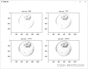
本文中采用高斯加权法进行局部阈值分割,并设置了5*5、7*7、11*11、13*13四种邻域范围,对比不同邻域下的分割效果。
算法步骤
- 图像灰度化
- 不同邻域下高斯加权法的局部阈值分割
- Matplotlib显示
结果
源代码
- def binary(self):
- win6 = tk.Toplevel(self.master)
- win6.title('阈值分割')
- win6.geometry('800x600')
- fig6 = plt.figure(figsize=(8, 6))
- canvas6 = FigureCanvasTkAgg(fig6, master=win6)
- canvas6.draw()
- canvas6.get_tk_widget().grid()
- # 读入中文路径
- img = cv2.imdecode(np.fromfile(self.entry, dtype=np.uint8), cv2.IMREAD_COLOR)
- plt.rcParams['font.sans-serif'] = ['SimHei']
- plt.rcParams['axes.unicode_minus'] = False
- gray = cv2.cvtColor(img, cv2.COLOR_RGB2GRAY)
- # 二值化
- binary1 = cv2.adaptiveThreshold(gray, 255, cv2.ADAPTIVE_THRESH_GAUSSIAN_C, cv2.THRESH_BINARY, 5, 5)
- binary2 = cv2.adaptiveThreshold(gray, 255, cv2.ADAPTIVE_THRESH_GAUSSIAN_C, cv2.THRESH_BINARY, 7, 5)
- binary3 = cv2.adaptiveThreshold(gray, 255, cv2.ADAPTIVE_THRESH_GAUSSIAN_C, cv2.THRESH_BINARY, 11, 5)
- binary4 = cv2.adaptiveThreshold(gray, 255, cv2.ADAPTIVE_THRESH_GAUSSIAN_C, cv2.THRESH_BINARY, 13, 5)
- ax3 = fig6.add_subplot(221)
- ax3.set_title('kernal 5*5')
- image1 = np.dstack([binary1, binary1, binary1])
- ax3.imshow(image1)
- ax4 = fig6.add_subplot(222)
- ax4.set_title('kernal 7*7')
- image2 = np.dstack([binary2, binary2, binary2])
- ax4.imshow(image2)
- ax5 = fig6.add_subplot(223)
- ax5.set_title('kernal 11*11')
- image3 = np.dstack([binary3, binary3, binary3])
- ax5.imshow(image3)
- ax6 = fig6.add_subplot(224)
- ax6.set_title('kernal 13*13')
- image4 = np.dstack([binary4, binary4, binary4])
- ax6.imshow(image4)
- # cv2.imwrite("image_binary.png", binary4)
5.3 Canny算子
Canny算子流程
- 高斯滤波去噪
- 计算梯度大小和梯度方向,其中梯度方向为
-
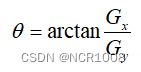
- 对梯度幅值图像进行非极大抑制(边缘的方向与梯度方向垂直)
- 双阈值处理和连接性分析确定边界
处理步骤
- 图像灰度化
- 高斯滤波处理
- 计算图像各方位的梯度大小和方向
- 对垂直于梯度方向的边缘进行非极大值抑制
- 进行双阈值处理和连结性分析确定边界
- Matplotlib显示
结果
源代码
- def boundary(self):
- win8 = tk.Toplevel(self.master)
- win8.title('Canny_boundary')
- win8.geometry('600x400')
- fig8 = plt.figure(figsize=(6, 4))
- canvas8 = FigureCanvasTkAgg(fig8, master=win8)
- canvas8.draw()
- canvas8.get_tk_widget().grid()
- img = cv2.imdecode(np.fromfile(self.entry, dtype=np.uint8), cv2.IMREAD_COLOR)
- gray = cv2.cvtColor(img, cv2.COLOR_BGR2GRAY)
- blurred = cv2.GaussianBlur(gray, (3, 3), 0)
- xgrad = cv2.Sobel(blurred, cv2.CV_16SC1, 1, 0)
- ygrad = cv2.Sobel(blurred, cv2.CV_16SC1, 0, 1)
- edge_output = cv2.Canny(xgrad, ygrad, 50, 150)
- edge_image = np.dstack([edge_output, edge_output, edge_output])
- ax1 = fig8.add_subplot(111)
- ax1.imshow(edge_image)
- ax1.set_title('Canny_boundary')
5.4区域生长
对于上述三种边缘提取的算法(Sobel算子、阈值分割、Canny算子)而言,可以分析得出:
- Sobel算子阴影处理效果不好,分界线不清晰
优点:输出图像(数组)的元素通常具有更大的绝对数值。
缺点:由于边缘是位置的标志,对灰度的变化不敏感。
- 自适应局部阈值法中,实验表明邻域为11*11时效果好,但斑点噪声多,不利于后处理。
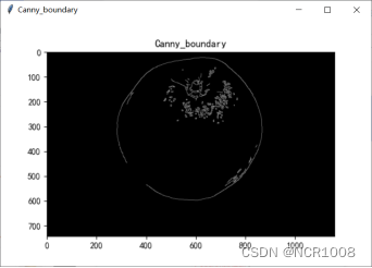
- Canny算子处理完之后为无阴影的二值图像,但部分边缘缺失。
优点:Canny算子增加了非极大值抑制以及双阈值方法,因此排除了非边缘点的干扰,检测效果更好,且标识出的边缘要与实际图像中的实际边缘尽可能接近。
缺点:图像中的边缘只能标识一次,并且可能存在的图像噪声不应标识为边缘。
就算对于效果最好的Canny算子而言,仍然存在一定的边缘缺失。因此我们考虑利用中心对称特性将其补全。
核心思想
由于在实际拍照过程中考虑到到光照等因素的原因,检测出的边缘会存在边缘缺失的情况,而为了提取出完整的边缘,我们需要对缺失部分进行补全。
又考虑到水果总是关于其中心对称的,因此沃恩可以采取判断每一个已知边缘点关于中心对称的点灰度值是否为255即可。
算法流程
- 执行Canny边缘提取
- 对提取后的数组进行遍历,求取其长、宽以及相对位置中心
- 构建与边缘提取后数组大小相同的新数组,并利用中心对称性对缺失值进行补全
- Matplotlib显示
结果
处理前: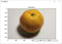
处理后: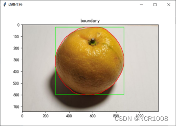
源代码
- def grow(self):
- # 生成新空间~
- win9 = tk.Toplevel(self.master)
- win9.title('边缘生长')
- win9.geometry('600x400')
- fig9 = plt.figure(figsize=(6, 4))
- canvas9 = FigureCanvasTkAgg(fig9, master=win9)
- canvas9.draw()
- canvas9.get_tk_widget().grid()
- # img[:,:,0]获取band1 shape:360,480
- img = cv2.imdecode(np.fromfile(self.entry, dtype=np.uint8), cv2.IMREAD_COLOR)
- gray = cv2.cvtColor(img, cv2.COLOR_BGR2GRAY)
- blurred = cv2.GaussianBlur(gray, (3, 3), 0)
- xgrad = cv2.Sobel(blurred, cv2.CV_16SC1, 1, 0)
- ygrad = cv2.Sobel(blurred, cv2.CV_16SC1, 0, 1)
- edge_output = cv2.Canny(xgrad, ygrad, 50, 150)
- # print(edge_output)
- width, height = edge_output.shape
- # print(width, height) # 360 480
- list_x = []
- list_y = []
- value = []
- for i in range(width):
- for j in range(height):
- if (edge_output[i][j] != 0):
- list_x.append(i)
- list_y.append(j)
- value.append(edge_output[i][j])
- # print(i, j)
- # print(edge_output[i][j])
- x_max = max(list_x)
- x_min = min(list_x)
- # print(x_max, x_min)
- x_mean = int((x_max + x_min) / 2)
- # print('x_mean', x_mean)
- y_max = max(list_y)
- y_min = min(list_y)
- img1 = cv2.rectangle(img, (y_min, x_min), (y_max, x_max), (0, 255, 0), 2) # 红
- y_mean = int((y_max + y_min) / 2)
- visited = np.zeros(shape=(edge_output.shape), dtype=np.uint8)
- for i in range(len(list_x)):
- x = list_x[i]
- y = list_y[i]
- # visited[x][y] = 1
- if x < x_mean and y < y_mean:
- directs = [(1, 0), (1, 1), (0, 1)]
- if x >= x_mean and y < y_mean:
- directs = [(-1, 0), (0, 1), (-1, 1)]
- if x < x_mean and y >= y_mean:
- directs = [(1, 0), (1, -1), (0, -1)]
- if x >= x_mean and y >= y_mean:
- directs = [(-1, 0), (-1, -1), (0, -1)]
- for direct in directs:
- current_x = x + direct[0]
- current_y = y + direct[1]
- if current_x < x_min or current_y < y_min or current_x >= x_max or current_y >= y_max:
- continue
- # if (not visited[current_x][current_y]) and (edge_output[current_x][current_y] == edge_output[x][y]):
- if (not visited[current_x][current_y]):
- edge_output[current_x][current_y] = 255
- visited[current_x][current_y] = 1
- x = 2 * x_mean - current_x
- y = 2 * y_mean - current_y
- # if(not visited[x][y] and current_y>y_mean and current_x<x_mean):
- if (not visited[x][y]):
- # 关于原点中心对称
- # 令关于远点对称点为(x,y)
- edge_output[x][y] = 255
- visited[x][y] = 1
-
- contours, heriachy = cv2.findContours(edge_output, cv2.RETR_EXTERNAL, cv2.CHAIN_APPROX_SIMPLE)
- max1 = 0
- maxA = 0
- print(contours, heriachy)
- for i, contour in enumerate(contours):
- x, y, w, h = cv2.boundingRect(contour)
- if w * h > maxA:
- max1 = i
- maxA = w * h
- cv2.drawContours(img1, contours, max1, (0, 0, 255), 2)
- band1 = img1[:, :, 0]
- band2 = img1[:, :, 1]
- band3 = img1[:, :, 2]
- ax1 = fig9.add_subplot(111)
- image = np.dstack([band3, band2, band1])
- ax1.imshow(image)
- ax1.set_title('boundary')
六、分类
| 边缘处理 | 区域生长 | Result | |
| Orange1 | 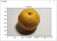 | 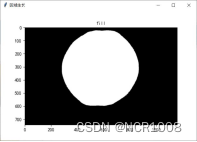 | 面积:597069 种类:橙子 |
| Orange2 | 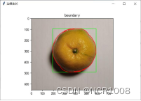 | 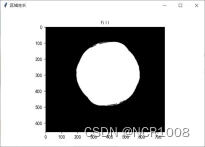 | 面积:362935 种类:橙子 |
| Lemon | 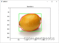 | 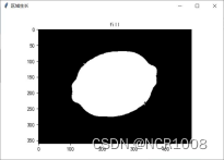 | 面积:130258 种类:柠檬 |

