
热门标签
热门文章
- 130天学会QT(进阶)--------------第二天(创建项目)
- 2嵌入式Linux开发环境搭建-(6)交叉编译QT4.8.7源码生成qmake工具
- 3【计算机网络】7. 网络基础5之详解以太网协议,ARP协议,NAT协议,DNS协议_arp和nat
- 4Mac 卸载重装 brew_mac 卸载brew
- 5$ionicView执行顺序_$scope.$on('$ionicview
- 6计算机启用远程桌面连接失败,开启局域网远程桌面连接不上怎么办
- 7Python文字识别_python识别文字
- 8flutter安卓模拟器不好使安卓每次打开android studio都下载并且download Importing ‘android“Gradle Project问题_importing android gradle project
- 9ARP协议,DNS协议,IP协议,TCP协议和IP路由原理
- 10几种使用了CNN(卷积神经网络)的文本分类模型_cnn文本分类模型是什么
当前位置: article > 正文
Python数据分析-4_plt.bar(range(len(_x)), _y)
作者:Gausst松鼠会 | 2024-03-15 19:42:38
赞
踩
plt.bar(range(len(_x)), _y)
1.对于一组电影数据,呈现出rating,runtime的分布情况:
- #encoding=utf-8
- import pandas as pd
- import numpy as np
- from matplotlib import pyplot as plt
- file_path = "./youtube_video_data/IMDB-Movie-Data.csv"
- df = pd.read_csv(file_path)
- #print(df.head(1))#读取第一行
- #print(df.info())#读取Data columns,显示数据条数
-
- #rating,runtime分布情况
- #选择图形,直方图
- #准备数据
- runtime_data = df["Runtime (Minutes)"].values
- #print(runtime_data)#读取运行时间的分钟数
- max_runtime = runtime_data.max()
- min_runtime = runtime_data.min()
- num_bin = (max_runtime - min_runtime)//10#显示直方图的组数
-
- #设置图形的大小
- plt.figure(figsize=(20,8),dpi=80)
- plt.hist(runtime_data,num_bin)#显示直方图
- plt.xticks(range(min_runtime,max_runtime+5,5))
- plt.show()
- #rating的显示类比以上代码

2.统计电影分类(genre)的情况(重新构造一个全为0的数组,列名为分类,如果一条数据中分类出现过,就让0变为1):
- #encoding=utf-8
- import pandas as pd
- import numpy as np
- from matplotlib import pyplot as plt
- file_path = "./youtube_video_data/IMDB-Movie-Data.csv"
- df = pd.read_csv(file_path)
- #print(df.head(1))
- #print(df["Genre"])#输出Genre的数据
- #统计分类的列表
- temp_list = df["Genre"].str.split(",").tolist()#[[],[],[]...]
- #print(temp_list)
- genre_list = list(set([i for j in temp_list for i in j]))
- #print(genre_list)
- #构造全为0的数组
- zeros_df = pd.DataFrame(np.zeros((df.shape[0],len(genre_list))),columns = genre_list)
- #print(df.shape[0])#输出的结果为行数1000
- #print(zeros_df)
-
- #给每个电影出现分类的位置赋值1
- for i in range(df.shape[0]):#遍历每一行
- #zeros_df.loc[0,["Sci-fi","Mucical"]] = 1
- zeros_df.loc[i,temp_list[i]] = 1 #把第i行,第temp_list[i]列的数设置为1
- #print(zeros_df.head(3))
- #统计每个分类的电影的数量和
- genre_count = zeros_df.sum(axis=0)
- #print(genre_count)
-
- #排序
- genre_count = genre_count.sort_values()
- _x = genre_count.index
- _y = genre_count.values
- #print(_x)
- #print(_y)
- #画图
- plt.figure(figsize=(20,8),dpi=80)
- plt.bar(range(len(_x)),_y)
- plt.xticks(range(len(_x)),_x)
- plt.show()
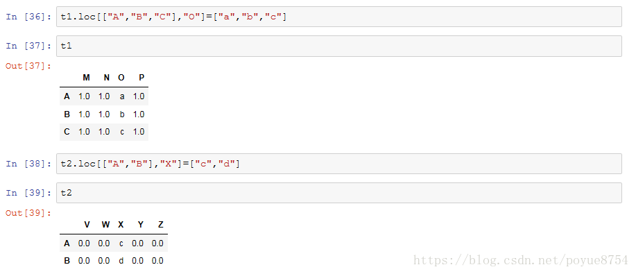
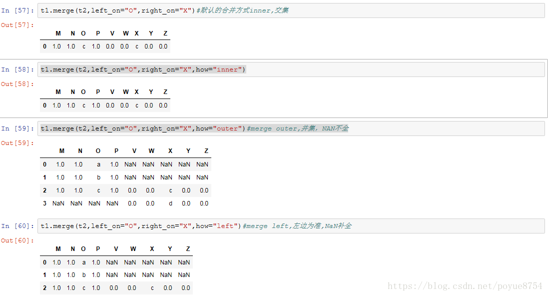
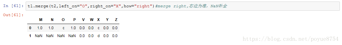
3.数据合并:
join : 默认情况下它是把行索引相同的数据合并到一起
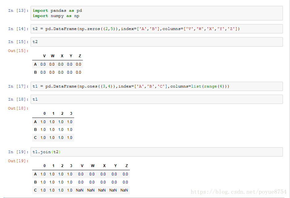
merge :按照指定的列把数据按照一定的方式合并到一起
4.全球星巴克店铺的统计数据,美国的星巴克数量和中国的哪个多,中国每个省份星巴克的数量:
- #encoding=utf-8
- import pandas as pd
- import numpy as np
- file_path = './youtube_video_data/starbucks_store_worldwide.csv'
- read_data = pd.read_csv(file_path)
- #print(read_data)
- #print(read_data.head(1))
- #print(read_data.info())
- grouped = read_data.groupby(by="Country")
- print(grouped)
- #DataFrameGroupBy
- #可以进行遍历
- # for i,j in grouped:
- # print(i)
- # print("-"*100)
- # print(j,type(j))
- # print("*"*100)
- #read_data[read_data["Country"]=="US"]
-
- #调用聚合方法,显示中国和美国的店铺数量
- #print(grouped["Brand"].count())
- # country_count = grouped["Brand"].count()
- # print(country_count["US"])
- # print(country_count["CN"])
-
- #统计中国每个省店铺的数量
- china_data = read_data[read_data["Country"] == "CN"]
- #print(china_data)
- grouped = china_data.groupby(by="State/Province").count()["Brand"]
- #print(grouped)
- df = read_data
- #数据按照多个条件进行分组
- grouped = df["Brand"].groupby(by=[(df["Country"]),df["State/Province"]]).count()
- # print(grouped)
- # print(type(grouped))
-
- #数据按照多个条件进行分组,返回DataFrame
- grouped1 = df["Brand"].groupby(by=[(df["Country"]),df["State/Province"]]).count()
- grouped2 = df.groupby(by=[df["Country"],df["State/Province"]])[["Brand"]].count()
- grouped3 = df.groupby(by=[df["Country"],df["State/Province"]]).count()[["Brand"]]
- # print(grouped1,type(grouped1))
- # print(grouped2,type(grouped2))
- # print(grouped3,type(grouped3))
- print(grouped1.index)
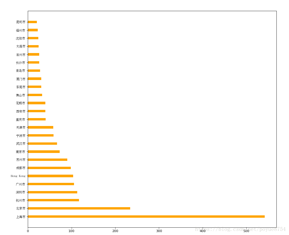
5.分组和聚合:


- # coding=utf-8
- import pandas as pd
- from matplotlib import pyplot as plt
- from matplotlib import font_manager
-
- my_font = font_manager.FontProperties(fname=r"c:\windows\fonts\simsun.ttc")
-
- file_path = "./youtube_video_data/starbucks_store_worldwide.csv"
-
- df = pd.read_csv(file_path)
- df = df[df["Country"]=="CN"]
-
- #使用matplotlib呈现出店铺总数排名前10的国家
- #准备数据
- data1 = df.groupby(by="City").count()["Brand"].sort_values(ascending=False)[:25]
-
- _x = data1.index
- _y = data1.values
-
- #画图
- plt.figure(figsize=(20,12),dpi=80)
-
- # plt.bar(range(len(_x)),_y,width=0.3,color="orange")
- plt.barh(range(len(_x)),_y,height=0.3,color="orange")
-
- plt.yticks(range(len(_x)),_x,fontproperties=my_font)
-
- plt.show()
显示结果:
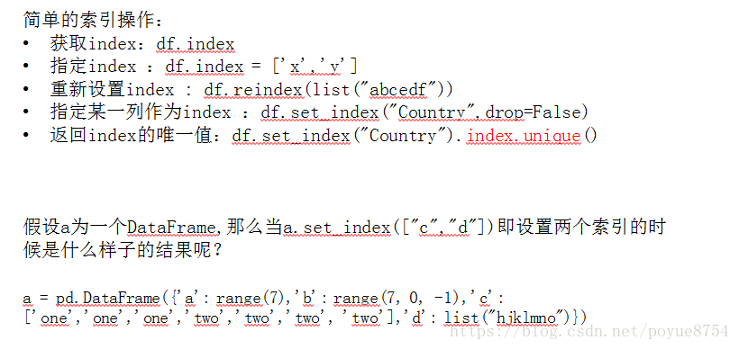
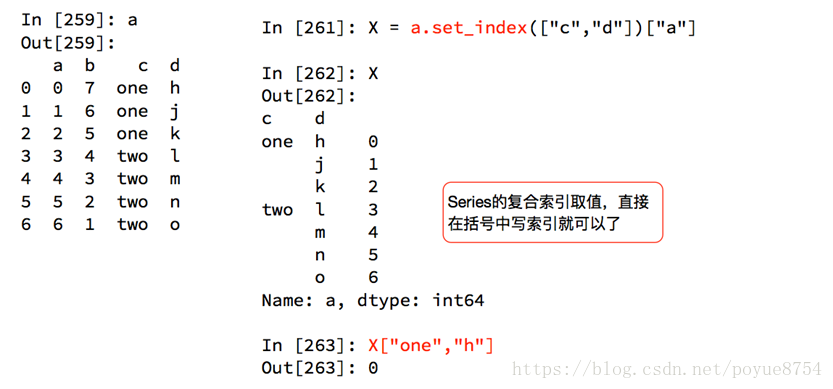
6.索引和复合索引:


6.有全球排名靠前的10000本书的数据,统计不同年份的数量,不同年份书的平均评分情况:
- #encoding=utf-8
- from matplotlib import pyplot as plt
- import numpy as np
- import pandas as pd
-
- file_path = "./youtube_video_data/books.csv"
- df = pd.read_csv(file_path)
- # print(df.head(2))
- # print(df.info())
- # data1 = df[pd.notnull(df["original_publication_year"])]
- # grouped = data1.groupby(by="original_publication_year").count().title
- # print(grouped)
- #不同年份书的平均评分情况
- #取出original_publication_year列中nan行
- data1 = df[pd.notnull(df["original_publication_year"])]
- grouped = data1["average_rating"].groupby(by=data1["original_publication_year"]).mean()
- #print(grouped)
-
- _x = grouped.index
- _y = grouped.values
- #画图
- plt.figure(figsize=(20,8),dpi=80)
- plt.plot(range(len(_x)),_y)
- plt.xticks(range(len(_x))[::10],_x[::10].astype(int),rotation=90)
- #plt.xticks(list(range(len(_x)))[::100],_x[::100],rotation=90)
- plt.show()
显示结果: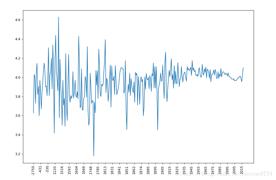
声明:本文内容由网友自发贡献,不代表【wpsshop博客】立场,版权归原作者所有,本站不承担相应法律责任。如您发现有侵权的内容,请联系我们。转载请注明出处:https://www.wpsshop.cn/w/Gausst松鼠会/article/detail/244052
推荐阅读
相关标签

