线性回归

1. 线性回归的定义

外事问谷歌,内事问百度。对于机器学习的重要概念的定义，我们需要去维基百科学习。原因在于两点，一为中文的翻译可能会误导人或者丢失一些重要知识点，二为百度百科中定义的内容良莠不齐。

先把维基百科的定义搬运过来：In statistics, linear regression is a linear approach to modelling the relationship between a scalar response (or dependent variable) and one or more explanatory variables (or independent variables).

在统计学中，线性回归是一种构建模型的线性方法，它描述的是单个输出的标量（因变量）和多个输入的解释变量（独立变量，被翻译成了自变量）之间的关系。到这里我得吐槽一句，不知道是谁把这个独立变量翻译成了自变量。看起来很简洁，但实际把重要的含义丢失了。在线性回归的后续学习中，会学到一个知识点：如果独立变量中存在多重共线性，就需要进行解决。（因为多重共线性就导致了dependent，而不是independent了。）

其中线性回归包括了单变量的线性回归和多元线性回归（multiple linear regression）。区别是独立变量的个数，前者独立变量个数为1，后者则大于1。在线性回归中，也存在因变量为多个的情况，称为是multivariate linear regression。很遗憾，百度百科写错了。（多元线性回归的英文名搞错了，写成了一个四不像的英文名~）

机器学习从参数这个维度来说，分为参数学习和非参数学习，其中参数学习中会用到参数估计方法。在线性回归中，使用线性函数对关系进行建模。其中线性函数中的未知参数是根据数据估计的。

Most commonly, the conditional mean of the response given the values of the explanatory variables (or predictors) is assumed to be an affine function of those values;less commonly, the conditional median or some other quantile is used.

由于因变量Y和独立变量X都是随机变量，对于每个确定的x值，Y都有它的分布。用F(Y|x)表示当x确定时，Y的概率分布函数。但是求F(Y|x)不是一件容易的事。所以我们采用近似的思想，不去求概率分布函数，而是求当x确定的时候，Y的期望或者中位数(E(Y))对应的函数，这样就把X和Y之间的关系转换成了$X和E(Y)$之间的关系，记为$\mu (x)$。

2. 线性回归证明

2.1 符号表示

首先我们将训练样本的特征矩阵X进行表示，其中N为样本个数，p为特征个数，每一行表示为每个样本，每一列表示特征的每个维度：
X = ( x 11 x 12 . . . x 1 p x 21 x 22 . . . x 2 p . . . . . . . . . . . . x N 1 x N 2 . . . x N p ) N ⋅ p X=

$$\begin{gathered} \begin{pmatrix} x_{11} & x_{12} & ... & x_{1p} \\ x_{21} & x_{22} & ... & x_{2p} \\ ... & ... &... &... \\ x_{N1} & x_{N2} & ... & x_{Np} \end{pmatrix} \quad \end{gathered}$$ _{N\cdot p} X= ​x11​x21​...xN1​​x12​x22​...xN2​​............​x1p​x2p​...xNp​​ ​​N⋅p​

然后我们对训练样本的标签向量Y和权重向量w进行表示，其中权重向量指的是线性回归中各个系数形成的向量。
Y = ( y 1 y 2 . . . y N ) Y =

$$\begin{gathered} \begin{pmatrix} y_{1} \\ y_{2} \\ ... \\ y_{N} \end{pmatrix} \quad \end{gathered}$$ Y= ​y1​y2​...yN​​ ​​

w = ( w 1 w 2 . . . w p ) w =

$$\begin{gathered} \begin{pmatrix} w_{1} \\ w_{2} \\ ... \\ w_{p} \end{pmatrix} \quad \end{gathered}$$ w= ​w1​w2​...wp​​ ​​
为了方便运算，我们把$y_i=x_{i}w+b$中的b也并入到w和x中。则上述的符号表示则为：

X = ( x 10 x 11 x 12 . . . x 1 p x 20 x 21 x 22 . . . x 2 p . . . . . . . . . . . . . . . x N 0 x N 1 x N 2 . . . x N p ) N ⋅ p X=

$$\begin{gathered} \begin{pmatrix} x_{10} & x_{11} & x_{12} & ... & x_{1p} \\ x_{20} & x_{21} & x_{22} & ... & x_{2p} \\ ... & ... &... &... &... \\ x_{N0} & x_{N1} & x_{N2} & ... & x_{Np} \end{pmatrix} \quad \end{gathered}$$ _{N\cdot p} X= ​x10​x20​...xN0​​x11​x21​...xN1​​x12​x22​...xN2​​............​x1p​x2p​...xNp​​ ​​N⋅p​

w = ( w 0 w 1 w 2 . . . w p ) w =

$$\begin{gathered} \begin{pmatrix} w_{0} \\ w_{1} \\ w_{2} \\ ... \\ w_{p} \end{pmatrix} \quad \end{gathered}$$ w= ​w0​w1​w2​...wp​​ ​​

2.2 公式推导

$$L(w)=\sum _{i=1}^N(x_{i}w-y_i{)}^2$$
$$w=\arg \min L(w)=\arg \min \sum _{i=1}^N(x_{i}w-y_i{)}^2$$
为什么是转置乘以原矩阵，这是由于Y是列向量，则$(XW-Y)$则也是列向量。根据矩阵乘法的定义，只有行向量乘以列向量，最终结果才是一个常数。
$$L(w)=(XW-Y{)}^T(XW-Y)$$

$$L(w)=(W^T{X}^T-Y^T)(XW-Y)$$

$$L(w)=(W^T{X}^{T}XW-2W^T{X}^{T}Y+Y^{T}Y)$$

$$\frac{\partial L(w)}{\partial w}=2X^{T}XW-2X^{T}Y=0$$

$$W={(X^{T}X)}^{-1}{X}^{T}Y$$

  后记：其实求非线性回归的时候也可以使用该最小二乘法来计算多项式系数$w$，只要把高次项添加到原始的$X$后面即可。

3. 代码实现

import numpy as np
from sklearn.metrics import r2_score

class LinearRegression:

    def __init__(self):
        
        self.coef_ = None
        self.intercept_ = None
        self._theta = None

    def fit(self, X_train, y_train):
    
        assert X_train.shape[0] == y_train.shape[0], \
            "the size of X_train must be equal to the size of y_train"

        X_b = np.hstack([np.ones((len(X_train), 1)), X_train])
        self._theta = np.linalg.inv(X_b.T.dot(X_b)).dot(X_b.T).dot(y_train)

        self.intercept_ = self._theta[0]
        self.coef_ = self._theta[1:]

        return self

    def predict(self, X_predict):
        assert self.intercept_ is not None and self.coef_ is not None, \
            "must fit before predict!"
        assert X_predict.shape[1] == len(self.coef_), \
            "the feature number of X_predict must be equal to X_train"

        X_b = np.hstack([np.ones((len(X_predict), 1)), X_predict])
        return X_b.dot(self._theta)

    def score(self, X_test, y_test):

        y_predict = self.predict(X_test)
        return r2_score(y_test, y_predict)
1
2
3
4
5
6
7
8
9
10
11
12
13
14
15
16
17
18
19
20
21
22
23
24
25
26
27
28
29
30
31
32
33
34
35
36
37

#生成数据
import numpy as np
#生成随机数
np.random.seed(1234)
x = np.random.rand(500,3)
#构建映射关系，模拟真实的数据待预测值,映射关系为y = 4.2 + 5.7*x1 + 10.8*x2，可自行设置值进行尝试
y = x.dot(np.array([4.2,5.7,10.8]))
1
2
3
4
5
6
7

from sklearn.linear_model import LinearRegression
import matplotlib.pyplot as plt
%matplotlib inline

# 调用模型
lr = LinearRegression(fit_intercept=True)
# 训练模型
lr.fit(x,y)
# 计算R平方
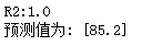
print('R2:%s' %(lr.score(x,y)))
# 任意设定变量，预测目标值
x_test = np.array([2,4,5]).reshape(1,-1)
y_hat = lr.predict(x_test)
print("预测值为: %s" %(y_hat))
1
2
3
4
5
6
7
8
9
10
11
12
13
14

linear_regression = LinearRegression()
linear_regression.fit(x, y)
x_test = np.array([2,4,5]).reshape(1,-1)
print('R2:%s' %(linear_regression.score(x,y)))
print("预测值为: %s" %(linear_regression.predict(x_test)))
1
2
3
4
5

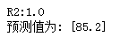
  可见自己实现的线性回归和sklearn中的线性回归是一致的。

4. 自回归(autoregressive)

  An autoregressive (AR) model is called autoregressive because it regresses the variable of interest against itself. In other words, it predicts the future value of a variable by using its past values. For example, an AR(1) model would use the value of the variable at the previous time step to predict its value at the current time step. An AR(2) model would use the values of the variable at the previous two time steps to predict its value at the current time step. And so on.

  所谓自回归模型隐含了是时间序列问题，因为有过去和未来，即有了时间轴。