《实战》基于情感词典的文本情感分析与LDA主题分析_not.csv

一、情感分析

1.1词典导入

import os
import numpy as np
import pandas as pd
import matplotlib.pyplot as plt
import seaborn as sns
from matplotlib.pylab import style #自定义图表风格
style.use('ggplot')
from IPython.core.interactiveshell import InteractiveShell
InteractiveShell.ast_node_interactivity = "all"
plt.rcParams['font.sans-serif'] = ['Simhei'] # 解决中文乱码问题

import re
import jieba.posseg as psg
import itertools
#conda install -c anaconda gensim
from gensim import corpora,models #主题挖掘，提取关键信息

# pip install wordcloud
from wordcloud import WordCloud,ImageColorGenerator
from collections import Counter

from sklearn.feature_extraction.text import CountVectorizer

review_long_clean = pd.read_excel('1_review_long_clean.xlsx')      #导入处理后的数据集
1
2
3
4
5
6
7
8
9
10
11
12
13
14
15
16
17
18
19
20
21
22
23
24

导入评价情感词典

#来自知网发布的情感分析用词语集

pos_comment=pd.read_csv('./正面评价词语（中文）.txt',header=None,sep='\n',encoding='utf-8') 
neg_comment=pd.read_csv('./负面评价词语（中文）.txt',header=None,sep='\n',encoding='utf-8')

pos_emotion=pd.read_csv('./正面情感词语（中文）.txt',header=None,sep='\n',encoding='utf-8')
neg_emotion=pd.read_csv('./负面情感词语（中文）.txt',header=None,sep='\n',encoding='utf-8')
1
2
3
4
5
6
7

查看一下正负情感词典分布

print('正面评价词语:',pos_comment.shape)
print('负面评价词语:',neg_comment.shape)

print('正面情感词语:',pos_emotion.shape)
print('负面情感词语:',neg_emotion.shape)
1
2
3
4
5

正面评价词语: (3743, 1)
负面评价词语: (3138, 1)
正面情感词语: (833, 1)
负面情感词语: (1251, 1)

#将正面和负面的合并
pos=pd.concat([pos_comment,pos_emotion],axis=0)
print('正面合并后:',pos.shape)

neg=pd.concat([neg_comment,neg_emotion],axis=0)
print('负面合并后:',neg.shape)
1
2
3
4
5
6

正面合并后: (4576, 1)
负面合并后: (4389, 1)

1.2 增加新词

#判断在不在词典中
c='点赞'
print(c in pos.values)

d='歇菜'
print(d in neg.values)
1
2
3
4
5
6

False
False

不在就添加进词典

#不在就添加进词典

new_pos=pd.Series(['点赞'])
new_neg=pd.Series(['歇菜'])

positive=pd.concat([pos,new_pos],axis=0)
print(positive.shape)

negative=pd.concat([neg,new_neg],axis=0)
print(negative.shape)
1
2
3
4
5
6
7
8
9
10

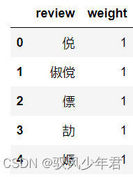
#将情感词存入，Dataframe中，并且正面词赋予权重1
positive.columns=['review']
positive['weight']=pd.Series([1]*len(positive))
positive.head()
1
2
3
4

#将情感词存入，Dataframe中，并且负面词赋予权重-1
negative.columns=['review']
negative['weight']=pd.Series([-1]*len(negative))
negative.head()
1
2
3
4

#将正负情感词合并
pos_neg=pd.concat([positive,negative],axis=0)
pos_neg.shape
1
2
3

(8967, 2)

1.3合并到review_long_clean中

#表联接
#清洗赶紧的数据，赋值给data
data=review_long_clean.copy()
print('data原始shape:',data.shape)

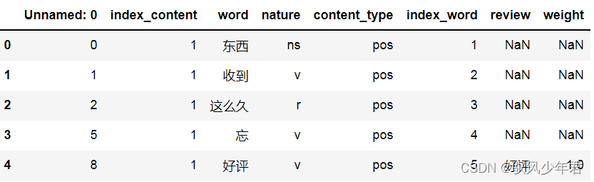
#将data和情感词两个表合并在一块，按照data的word列，情感数据按照review
review_mltype=pd.merge(data,pos_neg,how='left',left_on='word',right_on='review')
review_mltype.shape
print('表联接合并后：',review_mltype.shape)
print('----------完成评论中的情感词赋值------------')
print('review_mltype:')
review_mltype.head()
1
2
3
4
5
6
7
8
9
10
11
12

data原始shape: (25172, 6)
表联接合并后： (25172, 8)
----------完成评论中的情感词赋值------------
review_mltype:

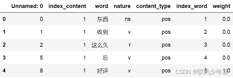
#删除情感值列，同时赋予不是情感词的词，权重为0
review_mltype=review_mltype.drop(['review'],axis=1)
review_mltype=review_mltype.replace(np.nan,0)
review_mltype.head()
1
2
3
4

1.4 修正情感倾向

如有多重否定，那么奇数否定是否定，偶数否定是肯定

看该情感词前2个词，来判罚否定的语气。如果在句首，则没有否词，如果在句子的第二次词，则看前1个词，来判断否定的语气。

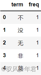
#读取否定词词典，新建一列为freq
notdict=pd.read_csv('./not.csv')
notdict.shape

notdict['freq']=[1]*len(notdict)
notdict.head()
1
2
3
4
5
6

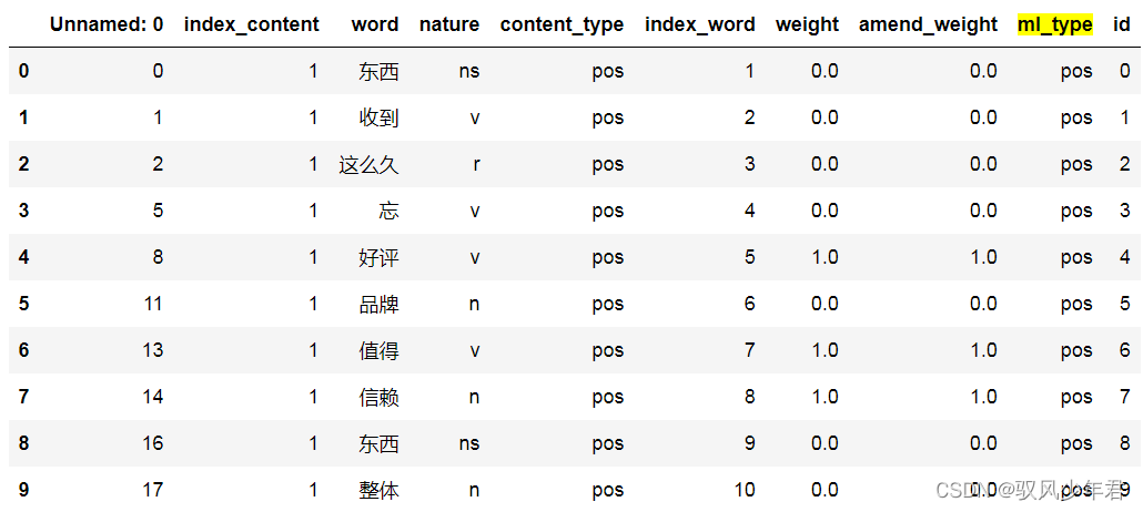
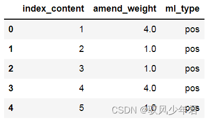
#准备一，构建amend_weight列，其值与情感权重值相同
review_mltype['amend_weight']=review_mltype['weight']
#创建，id列，初始化值为0-到最后一个的，顺序值
review_mltype['id']=np.arange(0,review_mltype.shape[0])
review_mltype.head(10)
1
2
3
4
5

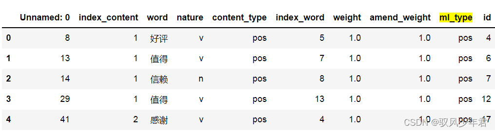
review_mltype是整理后有情感权重的，全部评论数据

只取出有情感值的文本

# 准备二，只取出有情感值的行
only_review_mltype=review_mltype[review_mltype['weight']!=0]

#只保留有情感值的索引
only_review_mltype.index=np.arange(0,only_review_mltype.shape[0]) #索引重置

print(only_review_mltype.shape)
only_review_mltype.head()
1
2
3
4
5
6
7
8

(1526, 10)

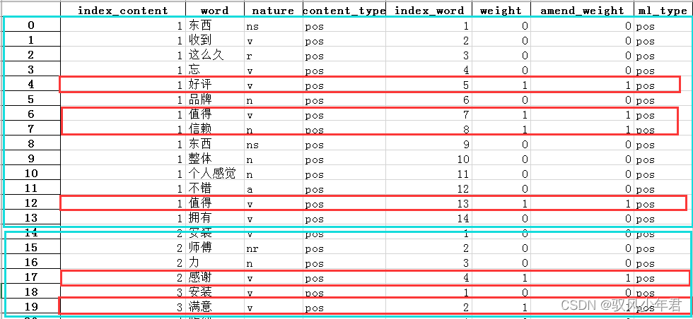
看该情感词前2个词，来判罚否定的语气。如果在句首，则没有否词，如果在句子的第二次词，则看前1个词，来判断否定的语气。

#看该情感词前2个词，来判罚否定的语气。如果在句首，则没有否词，如果在句子的第二次词，则看前1个词，来判断否定的语气。

index=only_review_mltype['id']

for i in range(0,only_review_mltype.shape[0]):
    
    review_i=review_mltype[review_mltype['index_content']==only_review_mltype['index_content'][i]] #第i个情感词的评论
    review_i.index=np.arange(0,review_i.shape[0])#重置索引后，索引值等价于index_word
    word_ind = only_review_mltype['index_word'][i] #第i个情感值在该条评论的位置
    
    #第一种，在句首。则不用判断
    #第二种，在评论的第2个为位置
    if word_ind==2:
        ne=sum( [ review_i['word'][word_ind-1] in notdict['term']  ] )
        if ne==1:
            review_mltype['amend_weight'][index[i]] = -( review_mltype['weight'][index[i]] )
    #第三种，在评论的第2个位置以后       
    elif word_ind > 2:
        ne=sum( [ word in notdict['term'] for word in review_i['word'][[word_ind-1,word_ind-2]]  ] ) # 注意用中括号[word_ind-1,word_ind-2]
        if ne==1:
            review_mltype['amend_weight'][index[i]]=- ( review_mltype['weight'][index[i]] )
1
2
3
4
5
6
7
8
9
10
11
12
13
14
15
16
17
18
19
20
21

review_mltype.shape
review_mltype[(review_mltype['weight']-review_mltype['amend_weight'])!=0] #说明两列值一样
1
2

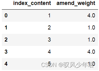
1.5计算每条评论的情感值

将一条文本中所有情感值计算，在相加到一块。

emotion_value=review_mltype.groupby('index_content',as_index=False)['amend_weight'].sum()
emotion_value.head()
emotion_value.to_csv('./1_emotion_value.csv',index=True,header=True)
1
2
3

1.6 查看情感分析效果

#每条评论的amend_weight总和不等于零

content_emotion_value=emotion_value.copy()
content_emotion_value.shape

#取出不等于0的的文本
content_emotion_value=content_emotion_value[content_emotion_value['amend_weight']!=0]

#设置情感倾向
content_emotion_value['ml_type']=''
content_emotion_value['ml_type'][content_emotion_value['amend_weight']>0]='pos'
content_emotion_value['ml_type'][content_emotion_value['amend_weight']<0]='neg'

content_emotion_value.shape
content_emotion_value.head()
1
2
3
4
5
6
7
8
9
10
11
12
13
14
15

二、情感分析效果

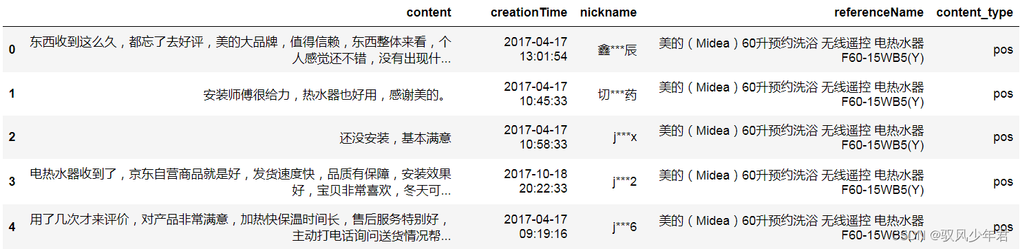
读取原始数据

#读取原始数据
raw_data=pd.read_csv('./reviews.csv')
raw_data.head()
1
2
3

方法缺陷：

#每条评论的amend_weight总和等于零
#这个方法其实不好用，有一半以上的评论区分不出正、负情感。

content_emotion_value0=emotion_value.copy()
content_emotion_value0=content_emotion_value0[content_emotion_value0['amend_weight']==0]
content_emotion_value0.head()

raw_data.content[6]
raw_data.content[7]
raw_data.content[8]

1
2
3
4
5
6
7
8
9
10
11

2.1 将数据合并

将情感分析结果，和原始数据集合并：

#合并到大表中

content_emotion_value=content_emotion_value.drop(['amend_weight'],axis=1)

review_mltype.shape

review_mltype=pd.merge(review_mltype,content_emotion_value,how='left',left_on='index_content',right_on='index_content')
review_mltype=review_mltype.drop(['id'],axis=1)
review_mltype.shape
review_mltype.head()

review_mltype.to_csv('./1_review_mltype',index=True,header=True)
1
2
3
4
5
6
7
8
9
10
11
12

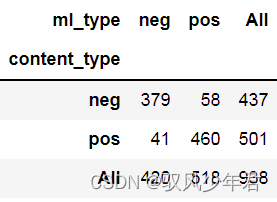
2.2 结果对比

与真实值对比下，情感分析结果的准确性：

cate=['index_content','content_type','ml_type']
data_type=review_mltype[cate].drop_duplicates()

confusion_matrix=pd.crosstab(data_type['content_type'],data_type['ml_type'],margins=True)
confusion_matrix
1
2
3
4
5

data=data_type[['content_type','ml_type']]
data=data.dropna(axis=0)
print( classification_report(data['content_type'],data['ml_type']) )
1
2
3

         precision    recall  f1-score   support
1

     neg       0.90      0.87      0.88       437
     pos       0.89      0.92      0.90       501
1
2

accuracy 0.89 938
macro avg 0.90 0.89 0.89 938
weighted avg 0.89 0.89 0.89 938

2.3 情感词云

将文本按照情感分类，然后统计词云

data=review_mltype.copy()

word_data_pos=data[data['ml_type']=='pos']
word_data_neg=data[data['ml_type']=='neg']

font=r"C:\Windows\Fonts\msyh.ttc"

background_image=plt.imread('./pl.jpg')
wordcloud = WordCloud(font_path=font, max_words = 100, mode='RGBA' ,background_color='white',mask=background_image) #width=1600,height=1200
wordcloud.generate_from_frequencies(Counter(word_data_pos.word.values))

plt.figure(figsize=(15,7))
plt.imshow(wordcloud)
plt.axis('off')
plt.show()

background_image=plt.imread('./pl.jpg')
wordcloud = WordCloud(font_path=font, max_words = 100, mode='RGBA' ,background_color='white',mask=background_image) #width=1600,height=1200
wordcloud.generate_from_frequencies(Counter(word_data_neg.word.values))

plt.figure(figsize=(15,7))
plt.imshow(wordcloud)
plt.axis('off')
plt.show()
1
2
3
4
5
6
7
8
9
10
11
12
13
14
15
16
17
18
19
20
21
22
23
24

三、基于LDA模型的主题分析

优点：不需要人工调试，用相对少的迭代找到最优的主题结构。

3.1建立词典、语料库

data=review_mltype.copy()

word_data_pos=data[data['ml_type']=='pos']
word_data_neg=data[data['ml_type']=='neg']
1
2
3
4

#建立词典，去重

pos_dict=corpora.Dictionary([ [i] for i in word_data_pos.word]) #shape=(n,1)
neg_dict=corpora.Dictionary([ [i] for i in word_data_neg.word])
1
2
3
4

#建立语料库
pos_corpus=[ pos_dict.doc2bow(j) for j in [ [i] for i in word_data_pos.word] ] #shape=(n,(2,1))
neg_corpus=[ neg_dict.doc2bow(j) for j in [ [i] for i in word_data_neg.word] ]
1
2
3

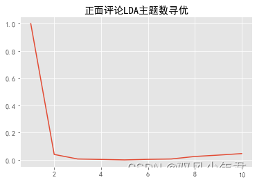
3.2主题数寻优

#构造主题数寻优函数

def cos(vector1,vector2):
    '''
    函数功能：余玄相似度函数
    '''
    dot_product=0.0
    normA=0.0
    normB=0.0
    for a,b in zip(vector1,vector2):
        dot_product +=a*b
        normA +=a**2
        normB +=b**2
    if normA==0.0 or normB==0.0:
        return None
    else:
        return ( dot_product/((normA*normB)**0.5) )
1
2
3
4
5
6
7
8
9
10
11
12
13
14
15
16
17

#主题数寻优
#这个函数可以重复调用，解决其他项目的问题

def LDA_k(x_corpus,x_dict):
    '''
    函数功能：
    '''
    #初始化平均余玄相似度
    mean_similarity=[]
    mean_similarity.append(1)
    
    #循环生成主题并计算主题间相似度
    for i in np.arange(2,11):
        lda=models.LdaModel(x_corpus,num_topics=i,id2word=x_dict) #LDA模型训练
        
        for j in np.arange(i):
            term=lda.show_topics(num_words=50)
        
        #提取各主题词
        top_word=[] #shape=(i,50)
        for k in np.arange(i):
            top_word.append( [''.join(re.findall('"(.*)"',i)) for i in term[k][1].split('+')]) #列出所有词
        
        #构造词频向量
        word=sum(top_word,[]) #列车所有词
        unique_word=set(word) #去重
        
        #构造主题词列表，行表示主题号，列表示各主题词
        mat=[] #shape=(i,len(unique_word))
        for j in np.arange(i):
            top_w=top_word[j]
            mat.append( tuple([ top_w.count(k) for k in unique_word ])) #统计list中元素的频次，返回元组
        
        #两两组合。方法一
        p=list(itertools.permutations(list(np.arange(i)),2)) #返回可迭代对象的所有数学全排列方式。
        y=len(p) # y=i*(i-1)
        top_similarity=[0]
        
        for w in np.arange(y):
            vector1=mat[p[w][0]]
            vector2=mat[p[w][1]]
            top_similarity.append(cos(vector1,vector2))

#        #两两组合，方法二
#        for x in range(i-1):
#            for y in range(x,i):
            
        #计算平均余玄相似度
        mean_similarity.append(sum(top_similarity)/ y)
    return mean_similarity
1
2
3
4
5
6
7
8
9
10
11
12
13
14
15
16
17
18
19
20
21
22
23
24
25
26
27
28
29
30
31
32
33
34
35
36
37
38
39
40
41
42
43
44
45
46
47
48
49
50

#计算主题平均余玄相似度

pos_k=LDA_k(pos_corpus,pos_dict)
neg_k=LDA_k(neg_corpus,neg_dict)

pos_k
neg_k

1
2
3
4
5
6
7
8

[1,
0.04,
0.006666666666666667,
0.0033333333333333335,
0.0,
0.004,
0.006666666666666666,
0.025000000000000015,
0.03500000000000002,
0.046222222222222234]
[1,
0.02,
0.0,
0.0,
0.0,
0.0026666666666666666,
0.002857142857142857,
0.0035714285714285718,
0.01333333333333334,
0.022222222222222233]

pd.Series(pos_k,index=range(1,11)).plot()
plt.title('正面评论LDA主题数寻优')
plt.show()
1
2
3

<matplotlib.axes._subplots.AxesSubplot at 0x1de4b888>
Text(0.5, 1.0, ‘正面评论LDA主题数寻优’)

pd.Series(neg_k,index=range(1,11)).plot()
plt.title('负面评论LDA主题数寻优')
plt.show()
1
2
3

matplotlib.axes._subplots.AxesSubplot at 0x1d077ac8>
Text(0.5, 1.0, ‘负面评论LDA主题数寻优’)

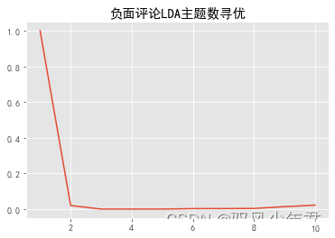
确定正负面主题数目都为3

pos_lda=models.LdaModel(pos_corpus,num_topics=2,id2word=pos_dict)
neg_lda=models.LdaModel(neg_corpus,num_topics=2,id2word=neg_dict)

pos_lda.print_topics(num_topics=10)
neg_lda.print_topics(num_topics=10)
1
2
3
4
5

[(0,
‘0.085*“安装” + 0.036*“满意” + 0.019*“服务” + 0.018*“不错” + 0.015*“好评” + 0.012*“客服” + 0.011*“人员” + 0.010*“物流” + 0.009*“送” + 0.008*“家里”’),
(1,
‘0.024*“师傅” + 0.021*“送货” + 0.019*“很快” + 0.016*“值得” + 0.013*“售后” + 0.012*“信赖” + 0.012*“东西” + 0.009*“太” + 0.009*“购物” + 0.009*“电话”’)]
[(0,
‘0.089*“安装” + 0.018*“师傅” + 0.015*“慢” + 0.013*“装” + 0.011*“打电话” + 0.011*“太慢” + 0.008*“坑人” + 0.008*“服务” + 0.007*“配件” + 0.007*“问”’),
(1,
‘0.021*“垃圾” + 0.019*“太” + 0.019*“差” + 0.016*“安装费” + 0.015*“售后” + 0.014*“东西” + 0.013*“不好” + 0.013*“客服” + 0.012*“加热” + 0.012*“小时”’)]