
热门标签
热门文章
- 1没时间了解技术热点?让大模型帮你整理重点吧!
- 2泛型(包装类),反射,枚举,lambda表达式_泛型枚举反射
- 3Docker Compose 通信超时问题及其解决方案_docker compose 超时
- 4java程序无法验证证书_Java没法验证,将不执行该应用程序
- 5Eureka 服务注册与发现_eureka auth 服务
- 6Shell逻辑判断、分支语句(带案例,Shell脚本学习笔记)_shell 条件判断 如何执行分支
- 7Docker与低代码跨平台开发:实现高效跨平台开发的新范式_docker 0代码平台
- 8CentOS 退出江湖,服务器操作系统该选择 Debian 还是 Ubuntu_centos ubuntu debian比较
- 9生成对抗网络(GAN)原理和实现_生成式对抗网络gan哪个论文提出
- 10推荐项目:Cordova 插件 Ionic Webview
当前位置: article > 正文
pytorch图像分类实战之构建数据集_pytorch数据集搭建过程
作者:煮酒与君饮 | 2024-06-24 00:45:17
赞
踩
pytorch数据集搭建过程
pytorch图像分类实战之构建数据集
前言
参加了一月份Datawale的组队学习,选择了pytorch图像分类实战的教程,主要是学习同济子豪兄的开源教程( https://space.bilibili.com/1900783/channel/collectiondetail?sid=606800 )。第一个任务是构建图像分类数据集。
1、环境配置
教程推荐使用云服务器来操作,实际演示也是按照云服务器的流程来的。教程推荐了云服务器租用平台,类似的平台还有很多,操作流程也都一样,按照教程便是使用jupyter lab来进行学习,不过基本都是付费的。配置好平台后,如果要使用教程的开源代码,直接利用jupyter lab运行就行了。
我使用的是AutoDL平台,刚开始注册送10元代金券就用了这个。

在自己电脑windows系统下也是能够运行教程的代码,实现效果的。不过肯定是不如云平台方便了。云GPU平台配置命令如下。
!pip install numpy pandas matplotlib requests tqdm opencv-python
- 1
2、图像采集
图像采集主要分为下载公开数据集、网络爬虫采集、自行拍摄三种方式。下载公开数据集与自行拍摄无需多少代码,而网络爬虫代码量较多,教程也给出了一套代码,实现爬虫采集图像的效果。下图是正在采集的过程。

下载已有数据集:
#melon17瓜果图像分类数据集
!wget https://zihao-openmmlab.obs.cn-east-3.myhuaweicloud.com/20220716-mmclassification/dataset/melon17/melon17_full.zip
#fruit81水果图像分类数据集
!wget https://zihao-openmmlab.obs.cn-east-3.myhuaweicloud.com/20220716-mmclassification/dataset/fruit81/fruit81_full.zip
- 1
- 2
- 3
- 4
3、数据集处理
(1) 删除多余文件
教程给出了删除系统自动生成的多余文件、删除gif格式图像文件、删除非三通道图像等方法来删掉数据集中的多余文件。
查看待删除的多余文件
!find . -iname '__MACOSX'
- 1
!find . -iname '.DS_Store'
- 1
!find . -iname '.ipynb_checkpoints'
./.ipynb_checkpoints
- 1
- 2
删除多余文件
!for i in `find . -iname '__MACOSX'`; do rm -rf $i;done
- 1
!for i in `find . -iname '.DS_Store'`; do rm -rf $i;done
- 1
!for i in `find . -iname '.ipynb_checkpoints'`; do rm -rf $i;done
- 1
验证多余文件已删除
!find . -iname '__MACOSX'
- 1
!find . -iname '.DS_Store'
- 1
!find . -iname '.ipynb_checkpoints'
- 1
删除gif格式的图像文件
dataset_path = 'dataset_delete_test'
- 1
for fruit in tqdm(os.listdir(dataset_path)):
    for file in os.listdir(os.path.join(dataset_path, fruit)):
        file_path = os.path.join(dataset_path, fruit, file)
        img = cv2.imread(file_path)
        if img is None:
            print(file_path, '读取错误,删除')
            os.remove(file_path)
- 1
- 2
- 3
- 4
- 5
- 6
- 7
删除非三通道的图像
import numpy as np
from PIL import Image
for fruit in tqdm(os.listdir(dataset_path)):
    for file in os.listdir(os.path.join(dataset_path, fruit)):
        file_path = os.path.join(dataset_path, fruit, file)
        img = np.array(Image.open(file_path))
        try:
            channel = img.shape[2]
            if channel != 3:
                print(file_path, '非三通道,删除')
                os.remove(file_path)
        except:
            print(file_path, '非三通道,删除')
            os.remove(file_path)
- 1
- 2
- 3
- 4
- 5
- 6
- 7
- 8
- 9
- 10
- 11
- 12
- 13
- 14
再次删除多余的.ipynb_checkpoints目录
!find . -iname '.ipynb_checkpoints'
./.ipynb_checkpoints
- 1
- 2
!for i in `find . -iname '.ipynb_checkpoints'`; do rm -rf $i;done
- 1
!find . -iname '.ipynb_checkpoints'
- 1
(2) 数据集划分
需要把数据集划分为训练集、测试集。
import os
import shutil
import random
import pandas as pd
# 指定数据集路径
dataset_path = 'fruit81_full'
dataset_name = dataset_path.split('_')[0]
print('数据集', dataset_name)
classes = os.listdir(dataset_path)
# 创建 train 文件夹
os.mkdir(os.path.join(dataset_path, 'train'))

# 创建 test 文件夹
os.mkdir(os.path.join(dataset_path, 'val'))

# 在 train 和 test 文件夹中创建各类别子文件夹
for fruit in classes:
    os.mkdir(os.path.join(dataset_path, 'train', fruit))
    os.mkdir(os.path.join(dataset_path, 'val', fruit))
test_frac = 0.2  # 测试集比例
random.seed(123) # 随机数种子,便于复现
df = pd.DataFrame()

print('{:^18} {:^18} {:^18}'.format('类别', '训练集数据个数', '测试集数据个数'))

for fruit in classes: # 遍历每个类别

    # 读取该类别的所有图像文件名
    old_dir = os.path.join(dataset_path, fruit)
    images_filename = os.listdir(old_dir)
    random.shuffle(images_filename) # 随机打乱

    # 划分训练集和测试集
    testset_numer = int(len(images_filename) * test_frac) # 测试集图像个数
    testset_images = images_filename[:testset_numer]      # 获取拟移动至 test 目录的测试集图像文件名
    trainset_images = images_filename[testset_numer:]     # 获取拟移动至 train 目录的训练集图像文件名

    # 移动图像至 test 目录
    for image in testset_images:
        old_img_path = os.path.join(dataset_path, fruit, image)         # 获取原始文件路径
        new_test_path = os.path.join(dataset_path, 'val', fruit, image) # 获取 test 目录的新文件路径
        shutil.move(old_img_path, new_test_path) # 移动文件

    # 移动图像至 train 目录
    for image in trainset_images:
        old_img_path = os.path.join(dataset_path, fruit, image)           # 获取原始文件路径
        new_train_path = os.path.join(dataset_path, 'train', fruit, image) # 获取 train 目录的新文件路径
        shutil.move(old_img_path, new_train_path) # 移动文件

    # 删除旧文件夹
    assert len(os.listdir(old_dir)) == 0 # 确保旧文件夹中的所有图像都被移动走
    shutil.rmtree(old_dir) # 删除文件夹

    # 工整地输出每一类别的数据个数
    print('{:^18} {:^18} {:^18}'.format(fruit, len(trainset_images), len(testset_images)))

    # 保存到表格中
    df = df.append({'class':fruit, 'trainset':len(trainset_images), 'testset':len(testset_images)}, ignore_index=True)

# 重命名数据集文件夹
shutil.move(dataset_path, dataset_name+'_split')

# 数据集各类别数量统计表格,导出为 csv 文件
df['total'] = df['trainset'] + df['testset']
df.to_csv('数据量统计.csv', index=False)

- 1
- 2
- 3
- 4
- 5
- 6
- 7
- 8
- 9
- 10
- 11
- 12
- 13
- 14
- 15
- 16
- 17
- 18
- 19
- 20
- 21
- 22
- 23
- 24
- 25
- 26
- 27
- 28
- 29
- 30
- 31
- 32
- 33
- 34
- 35
- 36
- 37
- 38
- 39
- 40
- 41
- 42
- 43
- 44
- 45
- 46
- 47
- 48
- 49
- 50
- 51
- 52
- 53
- 54
- 55
- 56
- 57
- 58
- 59
- 60
- 61
- 62
- 63
- 64
- 65
4、数据可视化
(1) 统计图像尺寸、比例分布
统计图像尺寸
代码:
df = pd.DataFrame()
for fruit in tqdm(os.listdir()): # 遍历每个类别
    os.chdir(fruit)
    for file in os.listdir(): # 遍历每张图像
        try:
            img = cv2.imread(file)
            df = df.append({'类别':fruit, '文件名':file, '图像宽':img.shape[1], '图像高':img.shape[0]}, ignore_index=True)
        except:
            print(os.path.join(fruit, file), '读取错误')
    os.chdir('../')
os.chdir('../')
- 1
- 2
- 3
- 4
- 5
- 6
- 7
- 8
- 9
- 10
- 11
结果:
| 类别 | 文件名 | 图像宽 | 图像高 | |
|---|---|---|---|---|
| 0 | 莲雾 | 63.jpg | 500.0 | 281.0 |
| 1 | 莲雾 | 189.jpg | 699.0 | 442.0 |
| 2 | 莲雾 | 77.jpg | 375.0 | 500.0 |
| 3 | 莲雾 | 162.jpg | 500.0 | 500.0 |
| 4 | 莲雾 | 176.jpg | 550.0 | 324.0 |
| … | … | … | … | … |
| 14428 | 腰果 | 147.jpg | 500.0 | 372.0 |
| 14429 | 腰果 | 52.jpg | 500.0 | 500.0 |
| 14430 | 腰果 | 46.jpg | 500.0 | 500.0 |
| 14431 | 腰果 | 190.jpg | 600.0 | 400.0 |
| 14432 | 腰果 | 184.jpg | 419.0 | 600.0 |
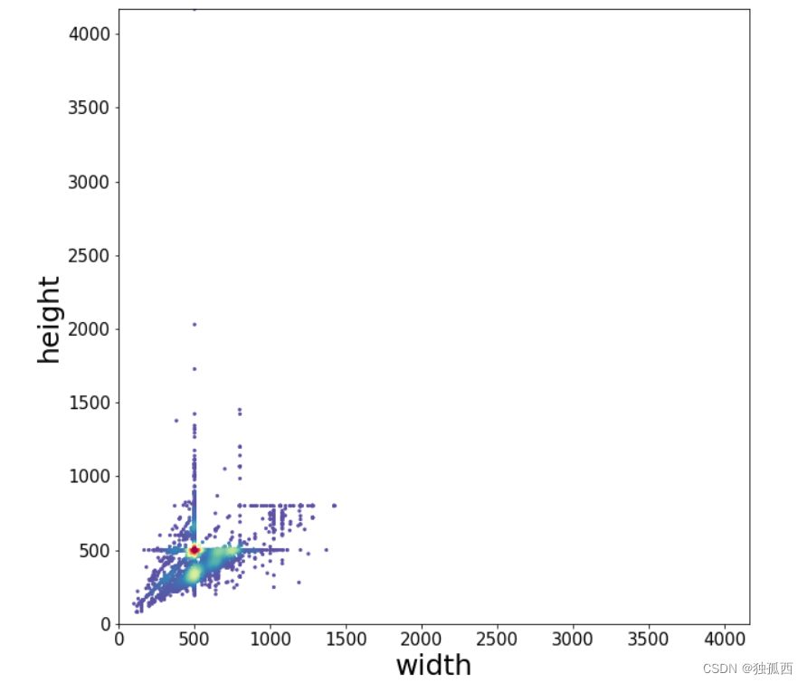
图像比例分布
代码:
from scipy.stats import gaussian_kde
from matplotlib.colors import LogNorm

x = df['图像宽']
y = df['图像高']

xy = np.vstack([x,y])
z = gaussian_kde(xy)(xy)

# Sort the points by density, so that the densest points are plotted last
idx = z.argsort()
x, y, z = x[idx], y[idx], z[idx]

plt.figure(figsize=(10,10))
# plt.figure(figsize=(12,12))
plt.scatter(x, y, c=z,  s=5, cmap='Spectral_r')
# plt.colorbar()
# plt.xticks([])
# plt.yticks([])

plt.tick_params(labelsize=15)

xy_max = max(max(df['图像宽']), max(df['图像高']))
plt.xlim(xmin=0, xmax=xy_max)
plt.ylim(ymin=0, ymax=xy_max)

plt.ylabel('height', fontsize=25)
plt.xlabel('width', fontsize=25)

plt.savefig('图像尺寸分布.pdf', dpi=120, bbox_inches='tight')

plt.show()
- 1
- 2
- 3
- 4
- 5
- 6
- 7
- 8
- 9
- 10
- 11
- 12
- 13
- 14
- 15
- 16
- 17
- 18
- 19
- 20
- 21
- 22
- 23
- 24
- 25
- 26
- 27
- 28
- 29
- 30
- 31
- 32
结果 :
(2) 可视化文件夹中的图像
代码:
import matplotlib.pyplot as plt
import matplotlib.image as mpimg
from mpl_toolkits.axes_grid1 import ImageGrid
%matplotlib inline

import numpy as np
import math
import os

import cv2

from tqdm import tqdm
folder_path = 'fruit81_split/train/桂圆'
# 可视化图像的个数
N = 36
# n 行 n 列
n = math.floor(np.sqrt(N))
images = []
for each_img in os.listdir(folder_path)[:N]:
    img_path = os.path.join(folder_path, each_img)
    img_bgr = cv2.imread(img_path)
    img_rgb = cv2.cvtColor(img_bgr, cv2.COLOR_BGR2RGB)
    images.append(img_rgb)
fig = plt.figure(figsize=(10, 10))
grid = ImageGrid(fig, 111,  # 类似绘制子图 subplot(111)
                 nrows_ncols=(n, n),  # 创建 n 行 m 列的 axes 网格
                 axes_pad=0.02,  # 网格间距
                 share_all=True
                 )

# 遍历每张图像
for ax, im in zip(grid, images):
    ax.imshow(im)
    ax.axis('off')

plt.tight_layout()
plt.show()
- 1
- 2
- 3
- 4
- 5
- 6
- 7
- 8
- 9
- 10
- 11
- 12
- 13
- 14
- 15
- 16
- 17
- 18
- 19
- 20
- 21
- 22
- 23
- 24
- 25
- 26
- 27
- 28
- 29
- 30
- 31
- 32
- 33
- 34
- 35
- 36
- 37
结果:

(3) 统计各类别图像数量
代码:
import numpy as np
import pandas as pd
import matplotlib.pyplot as plt
%matplotlib inline
df = pd.read_csv('数据量统计.csv')
# 指定可视化的特征
feature = 'total'
# feature = 'trainset'
# feature = 'testset'
plt.figure(figsize=(22, 7))

x = df['class']
y = df[feature]

plt.bar(x, y, facecolor='#1f77b4', edgecolor='k')

plt.xticks(rotation=90)
plt.tick_params(labelsize=15)
plt.xlabel('类别', fontsize=20)
plt.ylabel('图像数量', fontsize=20)

# plt.savefig('各类别图片数量.pdf', dpi=120, bbox_inches='tight')

plt.show()
plt.figure(figsize=(22, 7))
x = df['class']
y1 = df['testset']
y2 = df['trainset']

width = 0.55 # 柱状图宽度

plt.xticks(rotation=90) # 横轴文字旋转

plt.bar(x, y1, width, label='测试集')
plt.bar(x, y2, width, label='训练集', bottom=y1)


plt.xlabel('类别', fontsize=20)
plt.ylabel('图像数量', fontsize=20)
plt.tick_params(labelsize=13) # 设置坐标文字大小

plt.legend(fontsize=16) # 图例

# 保存为高清的 pdf 文件
plt.savefig('各类别图像数量.pdf', dpi=120, bbox_inches='tight')

plt.show()
- 1
- 2
- 3
- 4
- 5
- 6
- 7
- 8
- 9
- 10
- 11
- 12
- 13
- 14
- 15
- 16
- 17
- 18
- 19
- 20
- 21
- 22
- 23
- 24
- 25
- 26
- 27
- 28
- 29
- 30
- 31
- 32
- 33
- 34
- 35
- 36
- 37
- 38
- 39
- 40
- 41
- 42
- 43
- 44
- 45
- 46
- 47
结果:
| class | trainset | testset | total | |
|---|---|---|---|---|
| 0 | 莲雾 | 156.0 | 39.0 | 195.0 |
| 1 | 黄桃 | 155.0 | 38.0 | 193.0 |
| 2 | 圣女果 | 158.0 | 39.0 | 197.0 |
| 3 | 芒果 | 139.0 | 34.0 | 173.0 |
| 4 | 菠萝 | 158.0 | 39.0 | 197.0 |
| … | … | … | … | … |
| 76 | 金桔 | 145.0 | 36.0 | 181.0 |
| 77 | 红苹果 | 142.0 | 35.0 | 177.0 |
| 78 | 青柠 | 119.0 | 29.0 | 148.0 |
| 79 | 木瓜 | 156.0 | 38.0 | 194.0 |
| 80 | 腰果 | 160.0 | 40.0 | 200.0 |
81 rows × 4 columns


总结
本次学习主要是根据教程走了一遍流程,按部就班地进行了数据集的制作处理,没有大的改动。如果真正构建自己的数据集,可以通过爬虫下载好数据集,然后利用数据集处理部分的方法对数据集进行初步处理,之后再对数据集进行划分,然后可视化数据集,就完成了自己数据集的制作。
声明:本文内容由网友自发贡献,不代表【wpsshop博客】立场,版权归原作者所有,本站不承担相应法律责任。如您发现有侵权的内容,请联系我们。转载请注明出处:https://www.wpsshop.cn/w/煮酒与君饮/article/detail/751160
推荐阅读
相关标签

