可以选择与产品辛烷值(RON)非线性相关度较高的自变量，理论上互信息值较大的变量对于因变量的影响是较大的，是具有代表性的变量。但实际上，这些变量间相关性较高，即这些变量代表的可能是同一性质的操作，这一类性质的改变对于产品辛烷值的影响较大，所以它们的互信息量都处于较大的范围。为了使得选择的主要变量尽可能的具有代表性和独立性，所以需要在互信息分析的基础上去除掉自变量之间相关性高的部分，从而保证选择的变量不仅对因变量的相关度较高，而且各变量之间尽可能不相关，能够较为全面地代表操作变量整体。

我们这里使用matlab计算变量与产品辛烷值的互信息，选择互信息大的，在根据变量相关性，剔除相关性强的变量。


%计算两列向量之间的互信息
%u1：输入计算的向量1
%u2：输入计算的向量2
%wind_size：向量的长度
function mi = calmi(u1, u2, wind_size)
x = [u1, u2];
n = wind_size;
[xrow, xcol] = size(x);
bin = zeros(xrow,xcol);
pmf = zeros(n, 2);
for i = 1:2
    minx = min(x(:,i));
    maxx = max(x(:,i));
    binwidth = (maxx - minx) / n;
    edges = minx + binwidth*(0:n);
    histcEdges = [-Inf edges(2:end-1) Inf];
    [occur,bin(:,i)] = histc(x(:,i),histcEdges,1); %通过直方图方式计算单个向量的直方图分布
    pmf(:,i) = occur(1:n)./xrow;
end
%计算u1和u2的联合概率密度
jointOccur = accumarray(bin,1,[n,n]);  %（xi，yi）两个数据同时落入n*n等分方格中的数量即为联合概率密度
jointPmf = jointOccur./xrow;
Hx = -(pmf(:,1))'*log2(pmf(:,1)+eps);
Hy = -(pmf(:,2))'*log2(pmf(:,2)+eps);
Hxy = -(jointPmf(:))'*log2(jointPmf(:)+eps);
MI = Hx+Hy-Hxy;
mi = MI/sqrt(Hx*Hy);


clc
clear
load('origin.mat')
wind_size = size(data,1)
mi = zeros(354,1) ;
for i = 1 : 354 
    u1 = data(:,i);
    u2 = data(:,end);
    mi(i) = calmi(u1, u2, wind_size);
end
 
[res,index] = sort(mi,'descend')

二、Mann-Kendall 检验

2.1、M-K检验的理论知识

Mann-Kendall 检验法(M-K 法)是用于提取序列变化趋势的有效工具，也是“应用气候学实习”课程中重要的授课内容。

M-K 检验法最初由曼(H． B． Mann)和肯德尔(M．G． Kendall)提出了原理并发展了这一方法，是世界气象组织推荐的用于提取序列变化趋势的有效工具。M-K 检验法不受个别异常值的干扰，能够客观反映时间序列趋势，目前已经被广泛用于气候参数和水文序列的分析中。M-K 法可以根据输出的两个序列(UF和 UB)明确突变的时段和区域。

2.2、M-K检验的matlab实现


Data = [1961,4.7;
        1962,4.98;
        1963,5.39;
        1964,5.72;
        1965,4.88;
        1966,5.02;
        1967,5.1;
        1968,5.19;
        1969,4.31;
        1970,4.86;
        1971,5.28;
        1972,4.9;
        1973,5.23;
        1974,4.6;
        1975,5.88;
        1976,4.58;
        1977,5.37;
        1978,5.24;
        1979,4.91;
        1980,4.84;
        1981,4.98;
        1982,5.54;
        1983,5.67;
        1984,4.31;
        1985,4.67;
        1986,4.49;
        1987,4.96;
        1988,5.18;
        1989,5.41;
        1990,6.06;
        1991,5.4;
        1992,5.38;
        1993,5.3;
        1994,6.18;
        1995,5.58;
        1996,5.2;
        1997,5.8;
        1998,6.81;
        1999,6.47;
        2000,6;
        2001,6.16;
        2002,6.42;
        2003,6.7;
        2004,6.18;
        2005,5.52;
        2006,6.46;
        2007,6.73;
        2008,5.86;
        2009,5.61;
        2010,5.31;
        2011,5.69;
        2012,5.05;
        2013,5.13;
        2014,6.09;
        2015,6.13
        ] ;
y = Data(:,2);%平均温度序列
Sk = zeros(size(y)); % 定义累计量序列 Sk，长度 = y，初始值 =0，Sk(1) =0
UFk = zeros(size(y)); % 定义统计量 UFk，长度 = y，初始值 =0，UFk(1) =0
s = 0; % 定义 Sk 序列的元素 s
for i =2:length(y)
for j =1:i
if y(i) > y(j)
s = s +1;
else
s = s +0;
end
end
Sk(i) = s;
E = i* (i - 1) /4; % Sk(i)的均值，见式(3)
Var = i* (i - 1)* (2* i +5) /72; % Sk(i)方差，见式(3)
UFk(i) = (Sk(i)-  E) /sqrt(Var);% 正序列 UF 值，见式(2)
end
Sk2 = zeros(size(y)); % 定义逆序累计量序列 Sk2，长度= y，初始值 =0，Sk(2) =0
UBk = zeros(size(y)); % 定义逆序统计量 UBk，长度 = y，初始值 =0，UBk(1) =0
s =0;
y2 = flipud(y); % 按时间序列逆转平均温度序列
for i =2:length(y2)
for j =1:i
if y2(i) > y2(j)
s = s +1;
else
s = s +0;
end
end
Sk2(i) = s;
E = i* (i - 1) /4; %均值
Var = i* (i - 1)* (2* i +5) /72; %方差
UBk(i) = 0 - (Sk2(i) - E) /sqrt(Var);
end
UBk2 = flipud(UBk); %逆序列 UB 值
 
x = Data(:,1);%年份序列
n = length(x);%年份序列的长度
figure %做图
plot(x,UFk,'r-','linewidth',1.5);%画 UF 线
hold on
plot(x,UBk2,'b-.','linewidth',1.5);%画 UB 线
plot(x,1.96* ones(n,1),'k:','linewidth',1);
axis([min(x),max(x),-5,5]);%设置 X 轴范围和间距
legend('UF 统计量','UB 统计量','0.05 显著水平');% 设置图例
xlabel('年 Year','FontName','TimesNewRoman','FontSize',10);%X 轴标题
ylabel('统计量 MK Value','FontName','TimesNewRoman','Fontsize',10);%Y 轴标题
hold on
plot(x,-1.96 * ones(n,1),'k:','linewidth',1);
plot(x,0 * ones(n,1),'k-. ','linewidth',1);% 图片绘制

由图可知，该地区 1961 ～2015 年气温呈显著上升趋势，UF 和 UB 统计量有交点
且交点在置信直线范围之间，表明气温在 1989 年前后发生了突变。

三、小波分析

3.1、小波分析基本理论

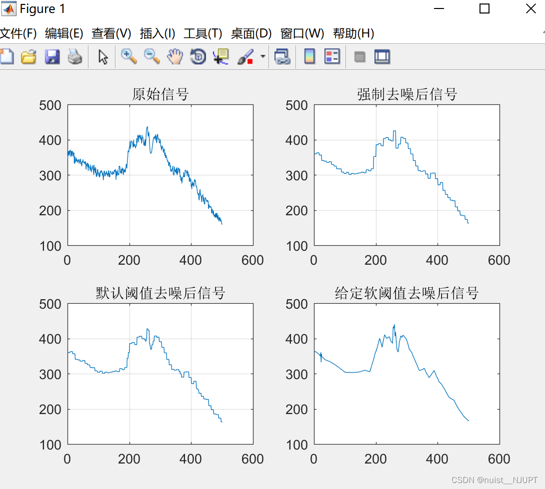
第一：去噪

小波分析的重要应用之一就是用于信号降噪。我们知道，一个含噪的一维信号模型可以表示为下图。其中s(k)为含噪信号，f(k)为有用信号，e(k)为噪声信号。这里我们认为e(k)是一个 1 级高斯白噪声，通常表现为高频信号，而实际工程中f(k)通常为低频信号或者是一些比较稳定的信号。

因此我们可按如下的方法进行降噪处理。首先对信号进行小波分解，一般地，噪声信号多包含在具有较高频率的细节中，从而，可利用门限阈值等形式对所分解的小波系数进行处理，然后对信号进行小波重构即可达到对信号降噪的目的。对信号降噪实质上是抑制信号中的无用部分，恢复信号中有用部分的过程。

小波信号降噪一般分为以下三个步骤：

(1)确定小波分解的层数，对信号进行分解。

(2)确定各个分解层下细节信号的阈值，对细节信号进行阈值量化处理。

(3)利用阈值处理后的细节信号和逼近信号进行重构，得到降噪后的信号。

第二：周期变化分析

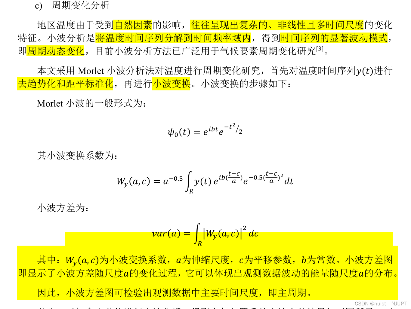
3.2、小波分析去噪matlab实现


 
clc;
clear all;
% 载入信号
% Load electrical signal and select a part of it.
load leleccum; 
indx = 2600:3100; 
 
%装载采集的信号
x = leleccum(indx);
lx=length(x);
t=[0:1:length(x)-1]';
 
%% 绘制监测所得信号
subplot(2,2,1);
plot(t,x);
title('原始信号');
grid on
%% 用db1小波对原始信号进行3层分解并提取小波系数
[c,l]=wavedec(x,3,'db1');
ca3=appcoef(c,l,'db1',3);
cd3=detcoef(c,l,3);
cd2=detcoef(c,l,2);
cd1=detcoef(c,l,1);
%% 对信号进行强制去噪处理并图示
cdd3=zeros(1,length(cd3));
cdd2=zeros(1,length(cd2));
cdd1=zeros(1,length(cd1));
c1=[ca3,cdd3,cdd2,cdd1];
x1=waverec(c1,l,'db1');
subplot(2,2,2);
plot(x1);
title('强制去噪后信号');
grid on
 
%% 默认阈值对信号去噪并图示%%
%用ddencmp( )函数获得信号的默认阈值，使用wdencmp( )函数实现去噪过程
[thr,sorh,keepapp]=ddencmp('den','wv',x);
x2=wdencmp('gbl',c,l,'db1',3,thr,sorh,keepapp);
subplot(2,2,3);
plot(x2);
title('默认阈值去噪后信号');
grid on
 
%% 给定的软阈值进行去噪处理并图示
wname = 'db3'; lev = 5;
[c,l] = wavedec(x,lev,wname);
alpha = 1.5; m = l(1);
[thr,nkeep] = wdcbm(c,l,alpha,m)
[xd,cxd,lxd,perf0,perfl2] = wdencmp('lvd',c,l,wname,lev,thr,'h');
subplot(2,2,4);
plot(xd);
title('给定软阈值去噪后信号');

3.3、小波分析周期变化分析matlab实现


%1.xiaozao函数，是需要对标准化的序列进行消除数据噪音分析；
%2.Db3函数，是对数列进行Db3趋势分析；
%3.period函数，是求得时间序列的实部和模的平方。
%其中周期变化图是实部的等值线图
%而小波方差是模的平方的算数平均。
clc
clear
close all;
load 暴雨量.mat
start_year=1958
 
a=s(:,1);
b=zscore(a);
scales=[1:1:32];
%进行连续小波变换得到小波系数矩阵,选择复morlet小波函数
wf=cwt(b,scales,'cmor1-1'); %计算小波系数
shibu=real(wf);% 求得系数的实部
mo=abs(wf); %计算小波系数模的绝对值
mofang=mo.^2; %计算小波系数的模方
fangcha=mean(mofang,2); %计算小波方差，小波方差是模的平方的算数平均
%**********画小波实部*************
figure(1);
j = j + 1;
% subplot(121);
% axis([1961,2015,0,50]);
width=713;%宽度，像素数
height=493;%高度
left=300;%距屏幕左下角水平距离
bottem=200;%距屏幕左下角垂直距离
set(gcf,'position',[left,bottem,width,height])
 
contourf(shibu,10,'-');
colormap('Jet');
colorbar;
hold on
set(gca,'FontSize',13,'Fontname', 'Times New Roman','Fontweight','bold');
xlabel('Year/a','FontName','Times new roman','FontSize',16,'Fontweight','bold');
ylabel('Scales/year','FontName','Times new roman','FontSize',16,'Fontweight','bold');
%set(gca,'XTick',1965:5:2017);
%set(gca,'XTicklabel', 1962:1:2017); %更新XTickLabel
set(gca,'xlim',[1 length(s)],'XTick',1:roundn(length(s)/5,0):length(s),'XTickLabel',start_year:roundn(length(s)/5,0):(start_year+length(s)-1))%修改横坐标的范围
title('(a)','Fontname','Times new roman','FontSize',18,'Fontweight','bold','position',[-4,52]);
%saveas(gca,[path_out5,num2str(j)],'png');
%close;
    
  
 
%********小波方差*************%
figure(2);
j = j + 1;
width=713;%宽度，像素数
height=493;%高度
left=300;%距屏幕左下角水平距离
bottem=200;%距屏幕左下角垂直距离
set(gcf,'position',[left,bottem,width,height])
  
% subplot(122);
plot(fangcha,'k-','linewidth',1.5);
set(gca,'FontName','Times new roman','FontSize',16,'Fontweight','bold');
xlabel('Scales/year','FontName','Times new roman','FontSize',16,'Fontweight','bold');
ylabel('Variance','FontName','Times new roman','FontSize',16,'Fontweight','bold');
title('(b)','Fontname','Times new roman','FontSize',18,'Fontweight','bold','position',[-3,1.8]);
set(gca,'XTick',0:5:31);
axis([1 32 0 2]);
grid on;   
%saveas(gca,[path_out5,num2str(j)],'png');
%close;
 
%********小波模**************%
figure(3);
j = j + 1;
%subplot(122);
width=713;%宽度，像素数
height=493;%高度
left=300;%距屏幕左下角水平距离
bottem=200;%距屏幕左下角垂直距离
set(gcf,'position',[left,bottem,width,height])
contourf(mo,10,'-');
colormap('Jet');
colorbar;
hold on
set(gca,'FontName','Times new roman','FontSize',13,'Fontweight','bold');   
xlabel('Year','FontName','Times new roman','FontSize',16,'Fontweight','bold');
ylabel('Scales/year','FontName','Times new roman','FontSize',16,'Fontweight','bold');
title('(c)','Fontname','Times new roman','FontSize',18,'Fontweight','bold','position',[-4,52]);
set(gca,'xlim',[1 length(s)],'XTick',1:roundn(length(s)/5,0):length(s),'XTickLabel',start_year:roundn(length(s)/5,0):(start_year+length(s)-1))
%saveas(gca,[path_out5,num2str(j)],'png');
%close;
    
%********小波模方**************%
figure(4);
j = j + 1;
%subplot(122);
width=713;%宽度，像素数
height=493;%高度
left=300;%距屏幕左下角水平距离
bottem=200;%距屏幕左下角垂直距离
set(gcf,'position',[left,bottem,width,height])
contourf(mofang,10,'-');
colormap('Jet');
colorbar;
hold on
set(gca,'FontName','Times new roman','FontSize',13,'Fontweight','bold');   
xlabel('Year','FontName','Times new roman','FontSize',16,'Fontweight','bold');
ylabel('Scales/year','FontName','Times new roman','FontSize',16,'Fontweight','bold');
set(gca,'xlim',[1 length(s)],'XTick',1:roundn(length(s)/5,0):length(s),'XTickLabel',start_year:roundn(length(s)/5,0):(start_year+length(s)-1))
%saveas(gca,[path_out5,num2str(j)],'png');

小波实部等值线图如下：

小波方差图如下：

小波模等值线图如下：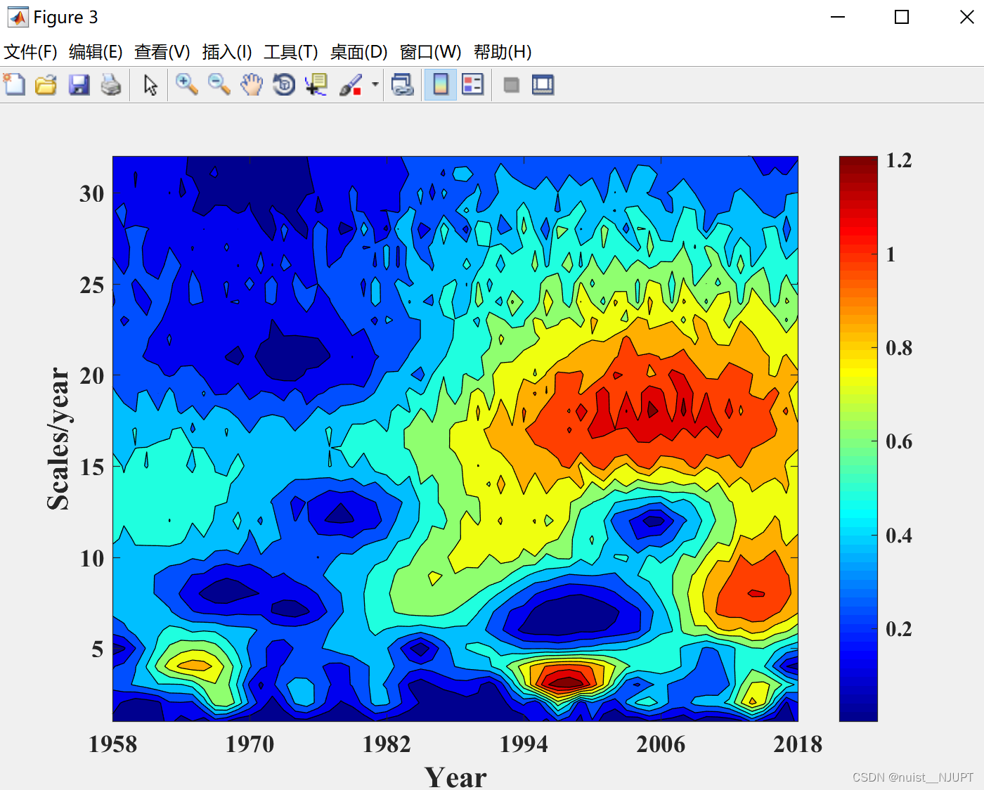

小波模方的等值线图：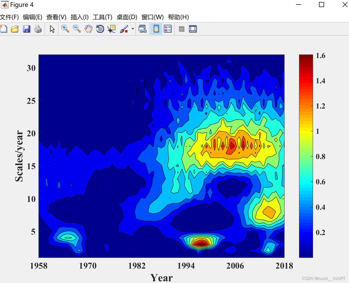

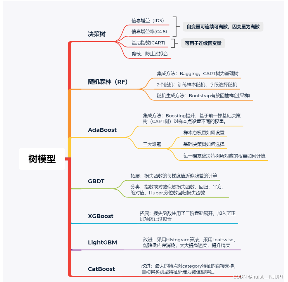
四、机器学习的常见树模型

由于之前的博客介绍了决策树和随机森林，这次主要介绍AdaBoost,GDBT,XGBoost,LigthGBM四种模型的理论及实现过程。

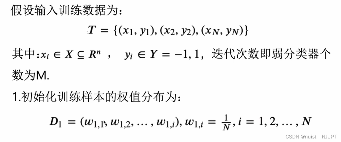
4.1、AdaBoost模型的基本思想和算法流程

Adaboost是一种迭代算法，其核心思想是针对同一个训练集训练不同的分类器(弱分类器)，然后把这些弱分类器集合起来，构成一个更强的最终分类器（强分类器）。

我们看一下Adaboost的模型，就是给分类误差小的分类器分配更多的权值，给分类误差大的分类器分配更大的权值。

我们看一下Adaboost的具体实现流程，首先输入训练样本x和y，然后初始化训练样本的权值分布，具体如下：

接下来进行遍历得到所有的弱分类器和所有的权值，具体如下：

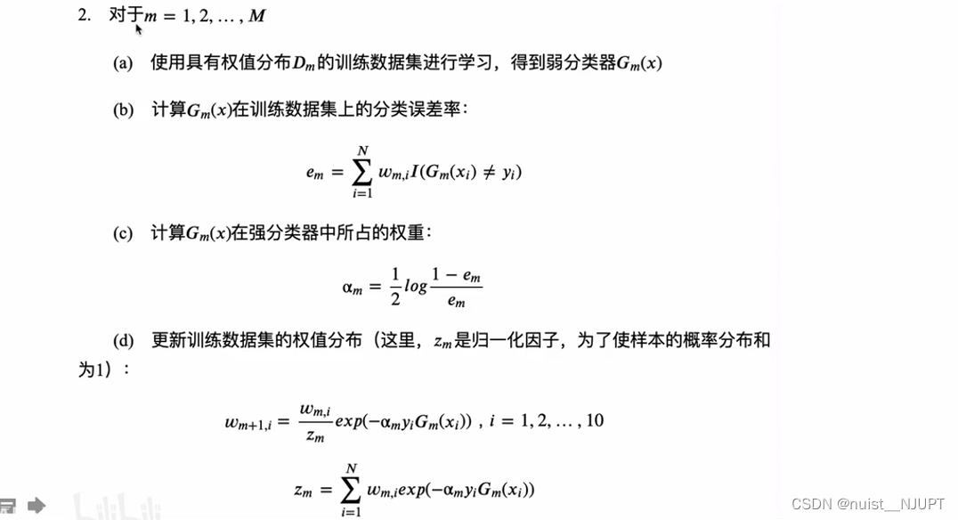
最后得到最终的分类器如下：

该算法其实是一个简单的弱分类算法提升过程，这个过程通过不断的训练，可以提高对数据的分类能力。整个过程如下所示：

1. 先通过对N个训练样本的学习得到第一个弱分类器；

2. 将分错的样本和其他的新数据一起构成一个新的N个的训练样本，通过对这个样本的学习得到第二个弱分类器；

3. 将1和2都分错了的样本加上其他的新样本构成另一个新的N个的训练样本，通过对这个样本的学习得到第三个弱分类器；

4. 最终经过提升的强分类器。即某个数据被分为哪一类要由各分类器权值决定。

4.2、AdaBoost模型的具体实现

下面使用python实现该模型的算法，完成一个二分类任务，我们使用Sklearn中的AdaBoost接口进行实践，具体如下：


import numpy as np
import matplotlib.pyplot as plt
from sklearn.ensemble import AdaBoostClassifier
from sklearn.tree import DecisionTreeClassifier
from sklearn.datasets import make_gaussian_quantiles
 
# 用make_gaussian_quantiles生成多组多维正态分布的数据
# 生成2维正态分布，设定样本数1000，协方差2
#其中x1是200行2列的数据,y1是200个输出样本表示分类结果
x1, y1 = make_gaussian_quantiles(
    cov=2., n_samples=200, n_features=2, n_classes=2, shuffle=True, random_state=1)
# 为了增加样本分布的复杂度，再生成一个数据分布
#x2是300行2列的数据,y2是300个输出样本表示分类结果
x2, y2 = make_gaussian_quantiles(mean=(
    3, 3), cov=1.5, n_samples=300, n_features=2, n_classes=2, shuffle=True, random_state=1)
 
#合并X水平合并，y竖直合并，然后按0和1不同颜色绘制散点图
X=np.vstack((x1,x2))
y=np.hstack((y1,1-y2))
# 绘制生成数据
plt.scatter(X[:,0],X[:,1],c=y)
plt.show()
 
#设定弱分类器CART
weakClassifier=DecisionTreeClassifier(max_depth=2)
#构建模型并进行训练
clf=AdaBoostClassifier(base_estimator=weakClassifier,algorithm='SAMME',n_estimators=300,learning_rate=0.8)
clf.fit(X, y)
 
# 模型预测
x1_min=X[:,0].min()-1
x1_max=X[:,0].max()+1
x2_min=X[:,1].min()-1
x2_max=X[:,1].max()+1
x1_,x2_=np.meshgrid(np.arange(x1_min,x1_max,0.02),np.arange(x2_min,x2_max,0.02))
y_=clf.predict(np.c_[x1_.ravel(),x2_.ravel()])
print(y)
 
# 结果绘制
#绘制分类效果
y_=y_.reshape(x1_.shape)
plt.contourf(x1_,x2_,y_,cmap=plt.cm.Paired)
plt.scatter(X[:,0],X[:,1],c=y)
plt.show()

原始的散点图与分类后的效果图如下：

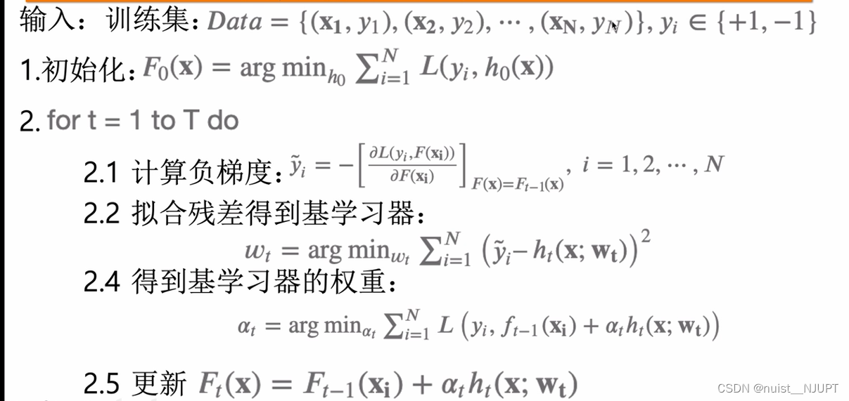
4.3、GBDT(梯度提升决策树)基本理论

我们看一下GDBT模型，就是梯度提升+决策树，利用损失函数的负梯度尽心你和学习器。

我们具体看一下为什么可以在GDBT模型中使用负梯度作为残差进行拟合，具体如下：

我们看一下这个GDBT的梯度提升的流程，具体如下：

4.4、XGBoost的基本理论

我们看一下XGBoost是GBBT模型的一种，XGBoost提供并行树提升（也称为GBDT，GBM），可以快速准确地解决许多数据科学问题。

我们先回顾一下决策树的概念，就是将不用的类别映射到叶子节点的概率进行分类和回归。

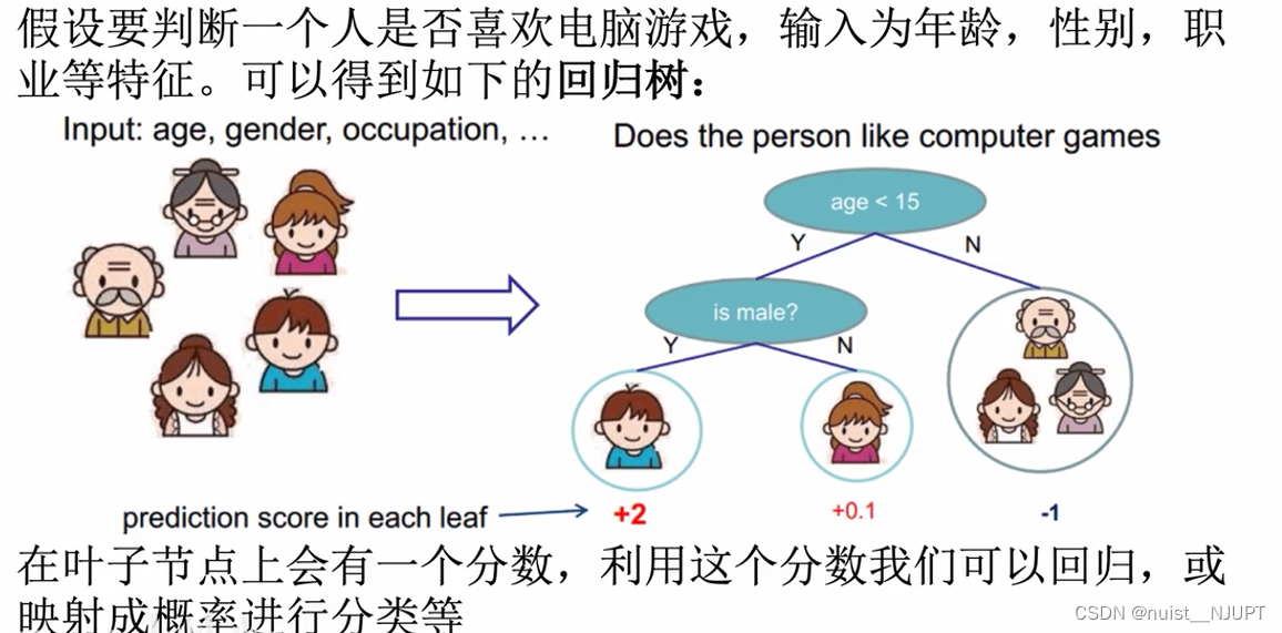
使用单个树进行集成学习的能力优先，一般考虑使用多棵树进行集成学习，就是随机森林或者提升树。

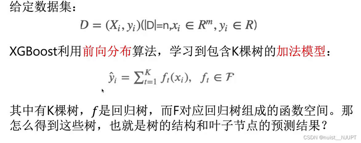
对于XGBoost的模型形式如下：是利用向前分布算法，学习到包含K棵树的加法模型。

4.5、XGBoost的实践(分类和回归)

分类问题，根据输入特征进行学习生成多个弱学习器，将多个弱学习器组合成一个强学习器，通过强学习器进行预测，输入的多组数据一共包含四个特征，输入的分类一共为3类：


import xgboost as xgb
from xgboost import plot_importance,plot_tree
from sklearn.datasets import load_iris
from sklearn.model_selection import train_test_split
from sklearn.metrics import accuracy_score
import matplotlib.pyplot as plt
 
# 加载样本数据集
#X有四个特征，y有三个类别:0,1,2
iris = load_iris()
X,y = iris.data,iris.target
 
# 获取特征名称:四个名称
feature_name = iris.feature_names
 
# 数据分割
X_train, X_test, y_train, y_test = train_test_split(X, y, test_size=0.2, random_state=3)
 
# 模型训练
model = xgb.XGBClassifier(max_depth=5, n_estimators=50, silent=True, objective='multi:softmax',feature_names=feature_name)
model.fit(X_train, y_train)
 
# 预测
y_pred = model.predict(X_test)
print(y_pred)
 
# 计算准确率
accuracy = accuracy_score(y_test,y_pred)
print("accuarcy: %.2f%%" % (accuracy*100.0))
 
# 显示重要特征
plot_importance(model)
plot_tree(model,num_trees=5)
plt.show()

测试集预测的结果如下，一共分为三类，即0，1，2.

四个特征的重要性排名如下：

绘制的决策树如下：

回归问题：

根据输入特征和输出特征进行回归，输入的多组数据的特征数目是9个，对结果进行预测，代码如下：


 
import xgboost as xgb
from xgboost import plot_importance,plot_tree
from sklearn.model_selection import train_test_split
from sklearn.datasets import load_boston
import matplotlib.pyplot as plt
 
# 获取数据
boston = load_boston()
X,y = boston.data,boston.target
 
 
# 数据集划分
X_train, X_test, y_train, y_test = train_test_split(X, y, test_size=0.2, random_state=0)
 
# 模型训练
model = xgb.XGBRegressor(max_depth=5, learning_rate=0.1, n_estimators=50, silent=True, objective='reg:gamma')
model.fit(X_train, y_train)
 
# 预测
y_pred = model.predict(X_test)
print(y_pred)
 
# 显示重要特征
plot_importance(model)
# 可视化树的生成情况，num_trees是树的索引
plot_tree(model, num_trees=17)
plt.show()

回归的预测结果如下：

对9个特征的重要性进行排名如下：

绘制的决策树如下所示：

五、支持向量机SVM

5.1、支持向量机基本理论

支持向量机（Support Vector Machine, SVM）是一类按监督学习（supervised learning）方式对数据进行二元分类的广义线性分类器（generalized linear classifier），其决策边界是对学习样本求解的最大边距超平面（maximum-margin hyperplane）。

支持向量机可以用于分类，回归预测和时间序列预测。

5.2、SVM实现持向量机回归(SVR)模型

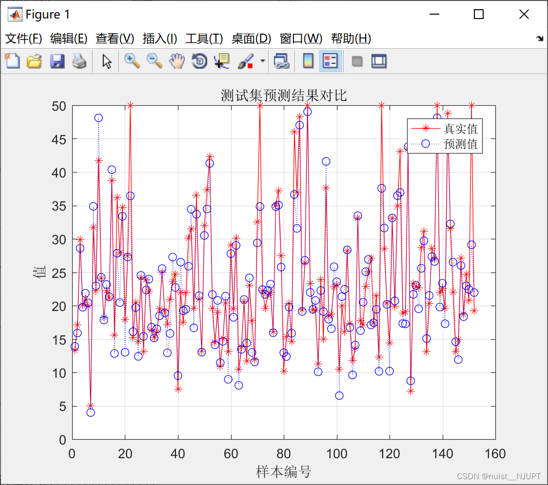
我们将数据划分为训练集和测试集，训练集有354组数据和13个特征，测试集是152组数据和13个特征，对数据进行回归预测，matlab的代码如下：


close all;
clc
clear
%% 下载数据
load('p_train.mat');
load('p_test.mat');
load('t_train.mat');
load('t_test.mat');
%% 数据归一化
%输入样本归一化
[pn_train,ps1] = mapminmax(p_train');
pn_train = pn_train';
pn_test = mapminmax('apply',p_test',ps1);
pn_test = pn_test';
%输出样本归一化
[tn_train,ps2] = mapminmax(t_train');
tn_train = tn_train';
tn_test = mapminmax('apply',t_test',ps2);
tn_test = tn_test';
%% SVR模型创建/训练
% 寻找最佳c参数/g参数——交叉验证方法
% SVM模型有两个非常重要的参数C与gamma。
% 其中 C是惩罚系数，即对误差的宽容度。
% c越高，说明越不能容忍出现误差,容易过拟合。C越小，容易欠拟合。C过大或过小，泛化能力变差
% gamma是选择RBF函数作为kernel后，该函数自带的一个参数。隐含地决定了数据映射到新的特征空间后的分布，
% gamma越大，支持向量越少，gamma值越小，支持向量越多。支持向量的个数影响训练与预测的速度。
[c,g] = meshgrid(-10:0.5:10,-10:0.5:10);
[m,n] = size(c);
cg = zeros(m,n);
eps = 10^(-4);
v = 5;
bestc = 0;
bestg = 0;
error = Inf;
for i = 1:m
    for j = 1:n
        cmd = ['-v ',num2str(v),' -t 2',' -c ',num2str(2^c(i,j)),' -g ',num2str(2^g(i,j) ),' -s 3 -p 0.1'];
        cg(i,j) = svmtrain(tn_train,pn_train,cmd);
        if cg(i,j) < error 
            error = cg(i,j);
            bestc = 2^c(i,j);
            bestg = 2^g(i,j);
        end
        if abs(cg(i,j) - error) <= eps && bestc > 2^c(i,j)
            error = cg(i,j);
            bestc = 2^c(i,j);
            bestg = 2^g(i,j);
        end
    end
end
% 创建/训练SVR 
cmd = [' -t 2',' -c ',num2str(bestc),' -g ',num2str(bestg),' -s 3 -p 0.01'];
model = svmtrain(tn_train,pn_train,cmd);
 
%% SVR仿真预测
% [Predict_1,error_1,dec_values_1] = svmpredict(tn_train,pn_train,model);
[Predict_2,error_2,dec_values_2] = svmpredict(tn_test,pn_test,model);
% 反归一化
% predict_1 = mapminmax('reverse',Predict_1,ps2);
predict_2 = mapminmax('reverse',Predict_2,ps2);
%% 计算误差
[len,~]=size(predict_2);
error = t_test - predict_2;
error = error';
MAE1=sum(abs(error./t_test'))/len;
MSE1=error*error'/len;
RMSE1=MSE1^(1/2);
R = corrcoef(t_test,predict_2);
r = R(1,2);
disp(['........支持向量回归误差计算................'])
disp(['平均绝对误差MAE为:',num2str(MAE1)])
disp(['均方误差为MSE:',num2str(MSE1)])
disp(['均方根误差RMSE为:',num2str(RMSE1)])
disp(['决定系数 R^2为:',num2str(r)])
figure(1)
plot(1:length(t_test),t_test,'r-*',1:length(t_test),predict_2,'b:o')
grid on
legend('真实值','预测值')
xlabel('样本编号')
ylabel('值')
string_2 = {'测试集预测结果对比'};
title(string_2)

预测效果如下：

5.3、SVM实现分类任务

下面是使用SVM实现对红酒分类的预测，一共187组数据，13个特征，输出的类别为3类。


%% Matlab神经网络43个案例分析
% 基于SVM的数据分类预测——意大利葡萄酒种类识别
%% 清空环境变量
close all;
clear;
clc;
format compact;
%% 数据提取
 
% 载入测试数据wine,其中包含的数据为classnumber = 3,wine:178*13的矩阵,wine_labes:178*1的列向量
load chapter_WineClass.mat;
 
% 画出测试数据的box可视化图
figure;
boxplot(wine,'orientation','horizontal','labels',categories);
title('wine数据的box可视化图','FontSize',12);
xlabel('属性值','FontSize',12);
grid on;
 
% 画出测试数据的分维可视化图
figure
subplot(3,5,1);
hold on
for run = 1:178
    plot(run,wine_labels(run),'*');
end
xlabel('样本','FontSize',10);
ylabel('类别标签','FontSize',10);
title('class','FontSize',10);
for run = 2:14
    subplot(3,5,run);
    hold on;
    str = ['attrib ',num2str(run-1)];
    for i = 1:178
        plot(i,wine(i,run-1),'*');
    end
    xlabel('样本','FontSize',10);
    ylabel('属性值','FontSize',10);
    title(str,'FontSize',10);
end
 
% 选定训练集和测试集
 
% 将第一类的1-30,第二类的60-95,第三类的131-153做为训练集
train_wine = [wine(1:30,:);wine(60:95,:);wine(131:153,:)];
% 相应的训练集的标签也要分离出来
train_wine_labels = [wine_labels(1:30);wine_labels(60:95);wine_labels(131:153)];
% 将第一类的31-59,第二类的96-130,第三类的154-178做为测试集
test_wine = [wine(31:59,:);wine(96:130,:);wine(154:178,:)];
% 相应的测试集的标签也要分离出来
test_wine_labels = [wine_labels(31:59);wine_labels(96:130);wine_labels(154:178)];
 
%% 数据预处理
% 数据预处理,将训练集和测试集归一化到[0,1]区间
 
[mtrain,ntrain] = size(train_wine);
[mtest,ntest] = size(test_wine);
 
dataset = [train_wine;test_wine];
% mapminmax为MATLAB自带的归一化函数
[dataset_scale,ps] = mapminmax(dataset',0,1);
dataset_scale = dataset_scale';
 
train_wine = dataset_scale(1:mtrain,:);
test_wine = dataset_scale( (mtrain+1):(mtrain+mtest),: );
%% SVM网络训练
tic;
model = svmtrain(train_wine_labels, train_wine, '-c 2 -g 1');
toc;
%% SVM网络预测
tic;
[predict_label, accuracy,dec_value1] = svmpredict(test_wine_labels, test_wine, model);
toc;
%% 结果分析
 
% 测试集的实际分类和预测分类图
% 通过图可以看出只有一个测试样本是被错分的
figure;
hold on;
plot(test_wine_labels,'o');
plot(predict_label,'r*');
xlabel('测试集样本','FontSize',12);
ylabel('类别标签','FontSize',12);
legend('实际测试集分类','预测测试集分类');
title('测试集的实际分类和预测分类图','FontSize',12);
grid on;

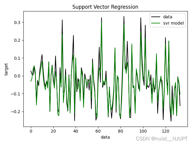
5.4、SVM实现时间序列预测

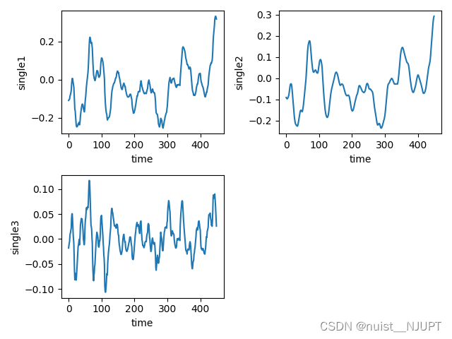
我们看一下SVM对于时间序列的预测，数据如下，第1列为时间，后面3列为时间的序列的数据，根据svm模型对时间序列数据进行预测，首先绘制B,C,D三类的时间序列变化图。

绘制出时间序列变化图，具体的时间序列变化如下所示，三组都是400个时间序列的样本数据。

模型训练与预测的代码如下，对测试集进行预测，绘制预测值和真实值的曲线，最后绘制预测误差的曲线。


#time时间列,single1,信号值,取前多少个X_data预测下一个数据
def time_slice(time,single,X_lag):
    sample = []
    label = []
    for k in range(len(time) - X_lag - 1):
        t = k + X_lag
        sample.append(single[k:t])
        label.append(single[t + 1])
    return sample,label
 
sample,label = time_slice(time,single1,5)
 
# 数据集划分
X_train, X_test, y_train, y_test = train_test_split(sample, label, test_size=0.3, random_state=42)
# 数据集掷乱
random_seed = 13
X_train, y_train = shuffle(X_train, y_train, random_state=random_seed)
# 参数设置SVR准备
parameters = {'kernel': ['rbf'], 'gamma': np.logspace(-5, 0, num=6, base=2.0),
              'C': np.logspace(-5, 5, num=11, base=2.0)}
# 网格搜索：选择十折交叉验证
svr = svm.SVR()
grid_search = GridSearchCV(svr, parameters, cv=10, n_jobs=4, scoring='neg_mean_squared_error')
# SVR模型训练
grid_search.fit(X_train, y_train)
# 输出最终的参数
print(grid_search.best_params_)
# 模型的精度
print(grid_search.best_score_)
# SVR模型保存
joblib.dump(grid_search, 'svr.pkl')
# SVR模型加载
svr = joblib.load('svr.pkl')
# SVR模型测试
y_hat = svr.predict(X_test)
# 计算预测值与实际值的残差绝对值
abs_vals = np.abs(y_hat - y_test)
 
plt.subplot(1, 1, 1)
plt.plot(y_test, c='k', label='data')
plt.plot(y_hat, c='g', label='svr model')
plt.xlabel('data')
plt.ylabel('target')
plt.title('Support Vector Regression')
plt.legend()
plt.show()
plt.subplot(1, 1, 1)
plt.plot(abs_vals)
plt.show()

使用训练好的svm模型进行预测值和真实值的拟合曲线图如下：

预测的值和真实值之间的误差变化图，具体如下：

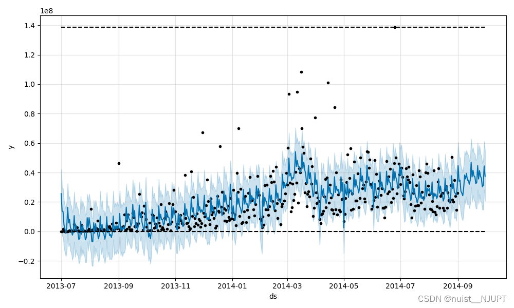
六、基于prophet的时间序列预测

6.1、prophet理论与实现一

我们可以看一下Prophet模型进行时间序列预测的基本模型，具体包括趋势项，周期项，节假日项，误差项，四个项目共同组成prophet模型。

我们根据原始时间序列数据去预测后30天的申购总额和赎回总额，原始数据是2013年7月到2014年的8月，我们使用当前的时间序列数据预测未来30天的，具体如下：

python代码实现如下：


import pandas as pd
import numpy as np
import matplotlib.pyplot as plt
from prophet import Prophet
from prophet.diagnostics import cross_validation
from prophet.diagnostics import performance_metrics
from prophet.plot import plot_cross_validation_metric
import warnings
warnings.filterwarnings('ignore')
 
#读取数据
data_user = pd.read_csv('user_balance_table.csv')
#将第一列的时间数据转换成固定格式
data_user['report_date'] = pd.to_datetime(data_user['report_date'], format='%Y%m%d')
#输出前面的头部信息
print(data_user.head())
 
#取时间列和另外要预测的两列
data_user_byday = data_user.groupby(['report_date'])['total_purchase_amt','total_redeem_amt'].sum().sort_values(['report_date']).reset_index()
print(data_user_byday.head())
 
 
# 定义模型
def FB(data: pd.DataFrame) -> pd.DataFrame:
    df = pd.DataFrame({
        'ds': data.report_date,
        'y': data.total_purchase_amt,
    })
 
    #申购总额的最大值和最小值
    df['cap'] = data.total_purchase_amt.values.max()
    df['floor'] = data.total_purchase_amt.values.min()
 
    m = Prophet(
        changepoint_prior_scale=0.05,
        daily_seasonality=False,
        yearly_seasonality=True,  # 年周期性
        weekly_seasonality=True,  # 周周期性
        growth="logistic",
    )
 
    m.add_seasonality(name='monthly', period=30.5, fourier_order=5, prior_scale=0.1)#月周期性
    m.add_country_holidays(country_name='CN')  # 中国所有的节假日
    m.fit(df)
    future = m.make_future_dataframe(periods=30, freq='D')  # 预测时长
    #预测的申购总额的最大值和最小值
    future['cap'] = data.total_purchase_amt.values.max()
    future['floor'] = data.total_purchase_amt.values.min()
    forecast = m.predict(future)
    fig = m.plot_components(forecast)
    fig1 = m.plot(forecast)
    return forecast
 
result_purchase = FB(data_user_byday)
print(result_purchase)
plt.show()

预测结果如下：

预测的周期性和趋势图等如下：

6.2、 prophet理论与实现二

数据部分，2013年7月到2014年8月的数据，对后30天的赎回总额进行预测，具体如下：

python代码如下：


import pandas as pd
import numpy as np
import matplotlib.pyplot as plt
from prophet import Prophet
from prophet.diagnostics import cross_validation
from prophet.diagnostics import performance_metrics
from prophet.plot import plot_cross_validation_metric
import warnings
warnings.filterwarnings('ignore')
 
#读取数据
data_user = pd.read_csv('user_balance_table.csv')
#将第一列的时间数据转换成固定格式
data_user['report_date'] = pd.to_datetime(data_user['report_date'], format='%Y%m%d')
#输出前面的头部信息
print(data_user.head())
 
#取时间列和另外要预测的两列
data_user_byday = data_user.groupby(['report_date'])['total_purchase_amt','total_redeem_amt'].sum().sort_values(['report_date']).reset_index()
print(data_user_byday.head())
 
# 定义模型
def FB(data: pd.DataFrame) -> pd.DataFrame:
 
    df = pd.DataFrame({
        'ds': data.report_date,
        'y': data.total_redeem_amt,
    })
 
    df['cap'] = data.total_redeem_amt.values.max()
    df['floor'] = data.total_redeem_amt.values.min()
 
    m = Prophet(
        changepoint_prior_scale=0.05,
        daily_seasonality=False,
        yearly_seasonality=True,  # 年周期性
        weekly_seasonality=True,  # 周周期性
        growth="logistic",
    )
    #365/12
    m.add_seasonality(name='monthly', period=30.5, fourier_order=5, prior_scale=0.1)  # 月周期性
    m.add_country_holidays(country_name='CN'  )  # 中国所有的节假日
 
    m.fit(df)
 
    future = m.make_future_dataframe(periods=30, freq='D'  )  # 预测时长
    future['cap'] = data.total_redeem_amt.values.max()
    future['floor'] = data.total_redeem_amt.values.min()
 
    forecast = m.predict(future)
 
    fig = m.plot_components(forecast)
    fig1 = m.plot(forecast)
 
    return forecast
result_redeem = FB(data_user_byday)
print(result_redeem)
plt.show()

预测结果如下：

周期性分析结果如下：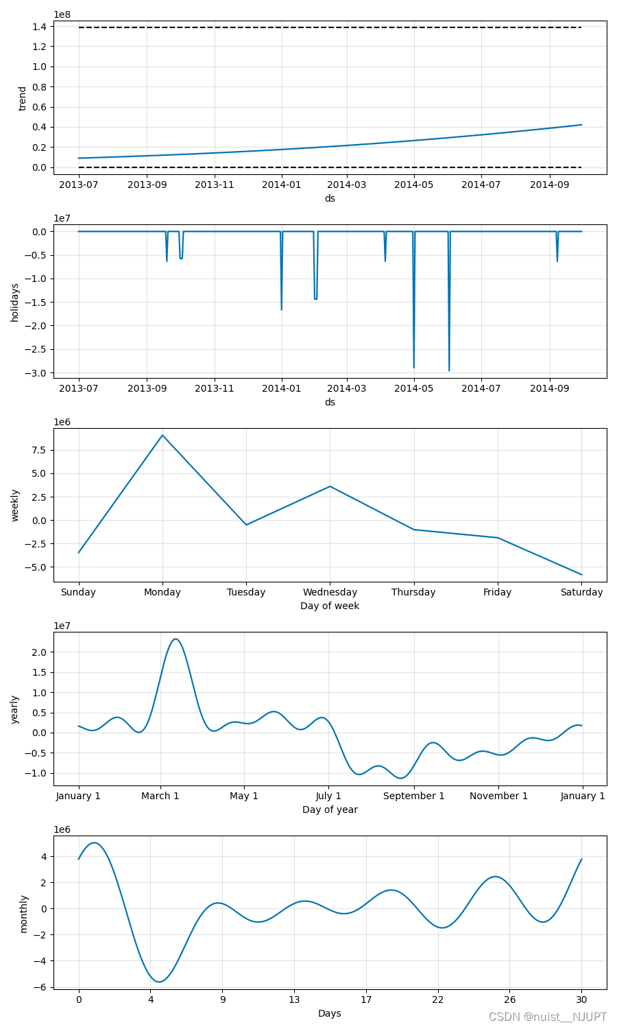

七、图像处理方法

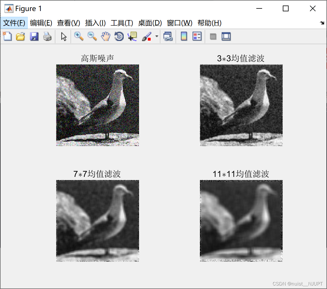
7.1、图像的去噪、增强

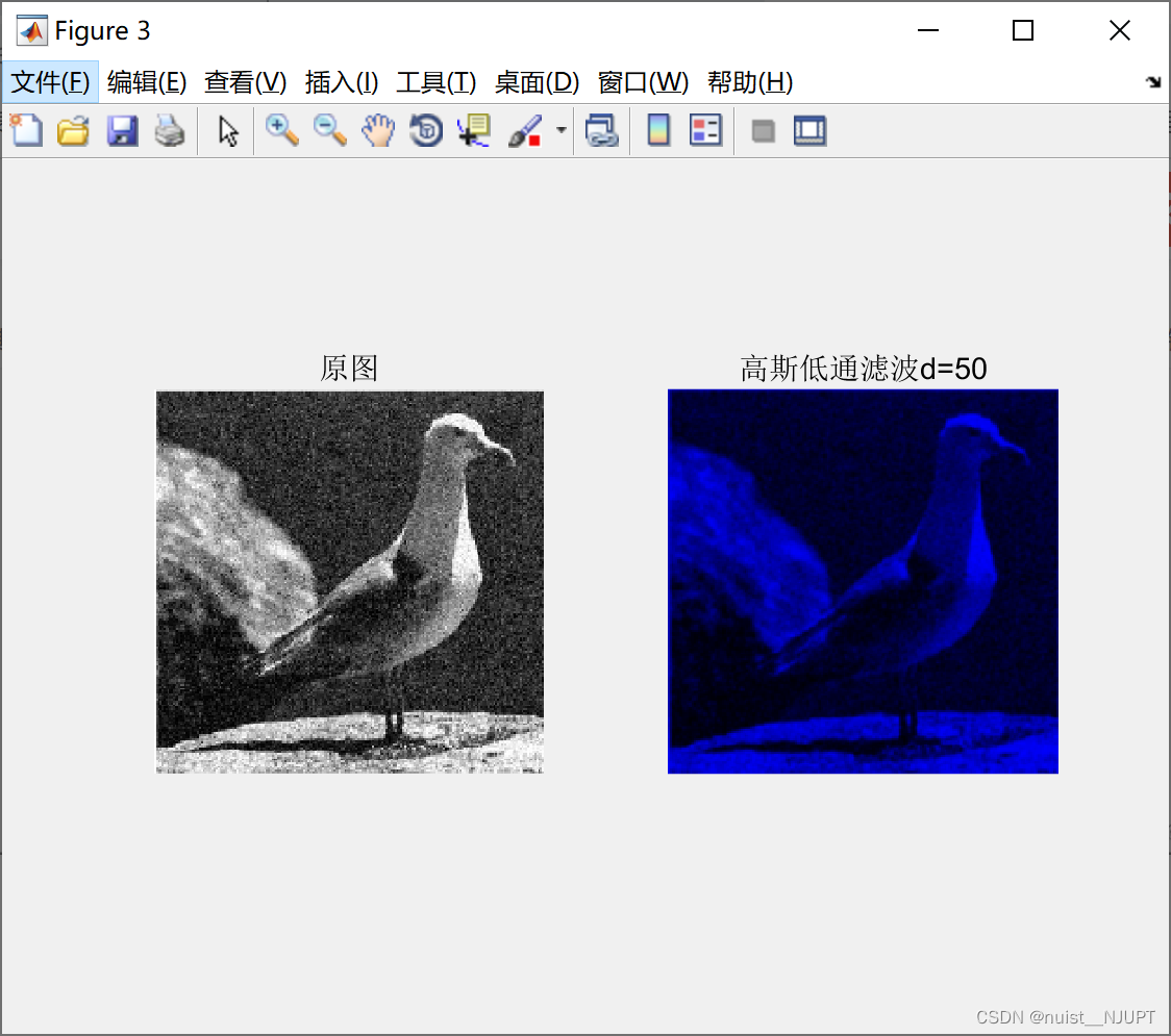
1、去噪是采用滤波的方式，本文使用了三种滤波方式：均值滤波，中值滤波，高斯高通滤波，滤波的主要代码如下，滤波的主要效果展示在图片中：


clear;
clc
g = imread('bird.jpg');
gg = imnoise(g, 'gaussian');  %添加高斯噪声
 
subplot(2,2,1);
imshow(gg); 
title('高斯噪声');
j = 2;
 
for i = 3:4:11
    subplot(2,2,j);
    G = avefilter(gg, i);
    imshow(G);
    title([num2str(i), '\ast', num2str(i), '均值滤波']);
    j = j+1;
end
 
figure(2);
g = imread('bird.png');
gg = imnoise(g, 'salt & pepper', 0.05); %添加椒盐噪声
 
subplot(2,2,1), imshow(gg); 
title('椒盐噪声');
 
j = 2;
for i = 3:4:11
    G = medianfilter(gg, i);
    subplot(2,2,j);
    imshow(G);
    title([num2str(i), '\ast', num2str(i), '中值滤波']);
    j = j+1;
end
 
figure(3);
d0=50;  %阈值
image=imread('bird.jpg');
[M,N,P] = size(image);
 
img_f = fft2(double(image));%傅里叶变换得到频谱
img_f=fftshift(img_f);  %移到中间
 
m_mid=floor(M/2);%中心点坐标
n_mid=floor(N/2);  
 
h = zeros(M,N,P);%高斯低通滤波器构造
for i = 1:M
    for j = 1:N
        d = ((i-m_mid)^2+(j-n_mid)^2);
        h(i,j) = exp(-d/(2*(d0^2)));      
    end
end
 
img_lpf = h.*img_f;
 
img_lpf=ifftshift(img_lpf);    %中心平移回原来状态
img_lpf=uint8(real(ifft2(img_lpf)));  %反傅里叶变换,取实数部分
 
subplot(1,2,1);
imshow(image);
title('原图');
subplot(1,2,2);
imshow(img_lpf);
title('高斯低通滤波d=50');


function G = avefilter(F, k)
% F 是待处理的图像
% k 是模版的大小,奇数
[m,n,p] = size(F) ;
 
% 转换数据类型，便于计算
G = uint16(zeros(m, n));
Ft = uint16(F);
M = uint16(ones(k, k));
h = (k+1)/2;
 
for i = 1:m
    for j = 1:n
        if((i < h)|| (j < h)|| (i > m-h+1)|| (j > n-h+1))   %不能被模版处理的区域
            G(i, j) = Ft(i, j); 
            continue;   %像素值不变
        end
        %取同样大小的图像块，中间的像素是待处理的像素
        T = Ft(i-(k-1)/2: i+(k-1)/2, j-(k-1)/2: j+(k-1)/2);
        T = T.*M;           %和模版相乘
        G(i, j) = sum(T(:))/k^2;    %结果求和并计算平均值
    end
end
G = uint8(G);       %结果转换成8-bit图像的数据类型


function G = medianfilter(F, k)
% F 是待处理的图像
% k 是模版的大小,奇数
[m,n,p] = size(F) ;
 
% 转换数据类型，便于计算
G = uint16(zeros(m, n)); Ft = uint16(F); M = uint16(ones(k, k));
h = (k+1)/2;
 
for i = 1:m
    for j = 1:n
        if((i < h)|| (j < h)|| (i > m-h+1)|| (j > n-h+1))   %不能被模版处理的区域
            G(i, j) = Ft(i, j); 
            continue;                   %像素值不变
        end
        % 取同样大小的图像块，中间的像素是待处理的像素
        T = Ft(i-(k-1)/2: i+(k-1)/2, j-(k-1)/2: j+(k-1)/2);
        T = T(:);               %将矩阵转换为一维向量
        G(i, j) = median(T);    %求中值并赋值给中间像素
    end
end
G = uint8(G);       %结果转换成8-bit图像的数据类型

滤波效果如下：

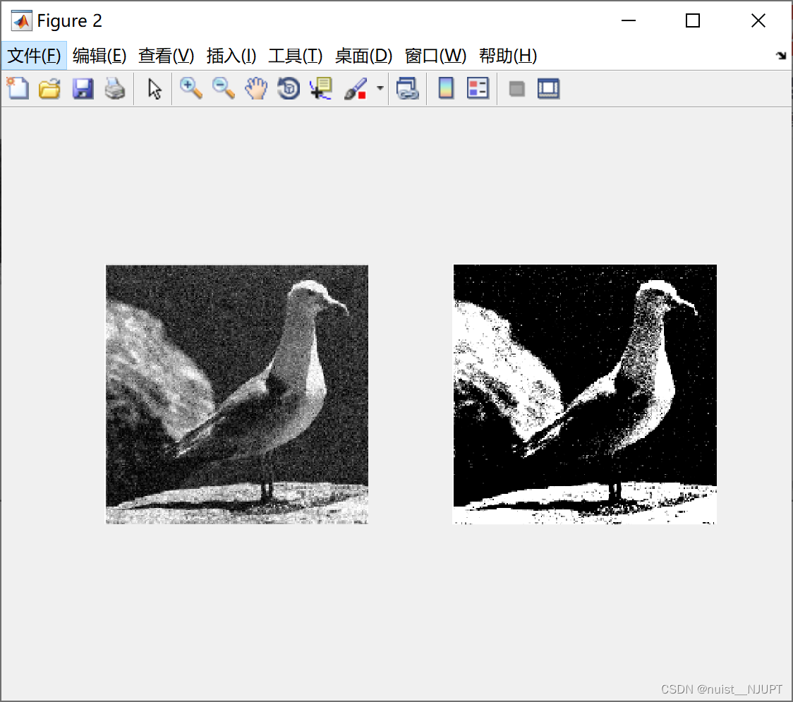
2-接下来对图像进行增强处理，主要采用两种方式，一种是灰度线性变换，另外一种是直方图均衡变换。

matlab实现灰度线性变换和直方图均衡变换进行图像增强的代码如下：


%% 获取灰色图像直方图
I = imread('bird.jpg'); %读取图片
I = rgb2gray(I); %把图片从rgb格式转为灰度图
 
row = size(I, 1); %获取图片像素的行列数
column = size(I, 2);
N = zeros(1, 256); %一个空的容器，用来记录每个像素出现的次数
 
% 两个循环用来遍历每一个像素
for i = 1:row
    for j = 1:column
        k = I(i, j); % 获取该像素点的像素值
        N(k + 1) = N(k + 1) + 1; % 记录下该像素值出现的次数
    end
end
 
%展示图片
figure(1);
subplot(121);imshow(I);
subplot(122);bar(N);
 
%% 灰色线性变换进行图像增强
I = imread('bird.jpg');
I = rgb2gray(I);
I = double(I);
 
J = (I - 80) * 255 / 70;
row = size(I, 1);
column = size(I, 2);
 
for i = 1:row
    for j = 1:column
        if J(i, j) < 0
            J(i, j) = 0;
        elseif J(i, j) > 255
            J(i, j) = 255;
        end
    end
end
 
figure(2);
subplot(121);imshow(uint8(I));
subplot(122);imshow(uint8(J));
 
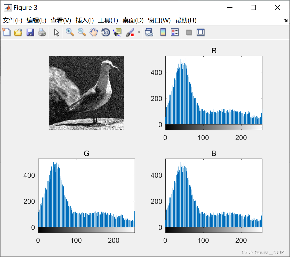
%% 直方图均衡变换进行图像增强
%R,G,B直方图展示
figure(3) ;
I = imread('bird.jpg');
subplot(221);imshow(I);
subplot(222);imhist(I(:, :, 1));title('R');
subplot(223);imhist(I(:, :, 2));title('G');
subplot(224);imhist(I(:, :, 3));title('B');
%均衡化方法
I = imread('bird.jpg');
G = rgb2gray(I) ;
J = histeq(G);
figure(4);
subplot(221);imshow(G);
subplot(222);imshow(J);
subplot(223);imhist(G);
subplot(224);imhist(J);

效果图如下：

原始图像和原始图像的灰色直方图如下：

对图像做了灰色线性变换后的图像对比如下：

原始图像的RGB直方图如下：

对原始图像做了直方图均衡变换的效果图：

7.2、图像特征提取

使用SITF算法进行图像特征提取，提取的特征位置如下，具体的matlab代码如下：

我们先看一下提取的效果：

主函数如下：


clear; 
clc
[image, descriptors, locs] = sift('deng.jpg');
disp('descriptors如下：') ;
disp(descriptors) ;
image1 = imread('deng.jpg');
showkeys(image1, locs)

sift算法函数如下：


% [image, descriptors, locs] = sift(imageFile)
%
% This function reads an image and returns its SIFT keypoints.
%   Input parameters:
%     imageFile: the file name for the image.
%
%   Returned:
%     image: the image array in double format
%     descriptors: a K-by-128 matrix, where each row gives an invariant
%         descriptor for one of the K keypoints.  The descriptor is a vector
%         of 128 values normalized to unit length.
%     locs: K-by-4 matrix, in which each row has the 4 values for a
%         keypoint location (row, column, scale, orientation).  The 
%         orientation is in the range [-PI, PI] radians.
%
% Credits: Thanks for initial version of this program to D. Alvaro and 
%          J.J. Guerrero, Universidad de Zaragoza (modified by D. Lowe)
 
function [image, descriptors, locs] = sift(imageFile)
 
% Load image
image1 = imread(imageFile);
image = rgb2gray(image1) ;
 
% If you have the Image Processing Toolbox, you can uncomment the following
%   lines to allow input of color images, which will be converted to grayscale.
% if isrgb(image)
%    image = rgb2gray(image);
% end
 
[rows, cols] = size(image); 
 
% Convert into PGM imagefile, readable by "keypoints" executable
f = fopen('tmp.pgm', 'w');
if f == -1
    error('Could not create file tmp.pgm.');
end
fprintf(f, 'P5\n%d\n%d\n255\n', cols, rows);
fwrite(f, image', 'uint8');
fclose(f);
% Call keypoints executable
if isunix
    command = '!./sift ';
else
    command = '!siftWin32 ';
end
command = [command ' <tmp.pgm >tmp.key'];
eval(command);
% Open tmp.key and check its header
g = fopen('tmp.key', 'r');
if g == -1
    error('Could not open file tmp.key.');
end
[header, count] = fscanf(g, '%d %d', [1 2]);
if count ~= 2
    error('Invalid keypoint file beginning.');
end
num = header(1);
len = header(2);
if len ~= 128
    error('Keypoint descriptor length invalid (should be 128).');
end
% Creates the two output matrices (use known size for efficiency)
locs = double(zeros(num, 4));
descriptors = double(zeros(num, 128));
% Parse tmp.key
for i = 1:num
    [vector, count] = fscanf(g, '%f %f %f %f', [1 4]); %row col scale ori
    if count ~= 4
        error('Invalid keypoint file format');
    end
    locs(i, :) = vector(1, :);
    
    [descrip, count] = fscanf(g, '%d', [1 len]);
    if (count ~= 128)
        error('Invalid keypoint file value.');
    end
    % Normalize each input vector to unit length
    descrip = descrip / sqrt(sum(descrip.^2));
    descriptors(i, :) = descrip(1, :);
end
fclose(g);

特征点的展示函数如下：


% showkeys(image, locs)
%
% This function displays an image with SIFT keypoints overlayed.
%   Input parameters:
%     image: the file name for the image (grayscale)
%     locs: matrix in which each row gives a keypoint location (row,
%           column, scale, orientation)
 
function showkeys(image, locs)
 
disp('Drawing SIFT keypoints ...');
 
% Draw image with keypoints
figure('Position', [50 50 size(image,2) size(image,1)]);
colormap('gray');
imagesc(image);
hold on;
imsize = size(image);
for i = 1: size(locs,1)
    % Draw an arrow, each line transformed according to keypoint parameters.
    TransformLine(imsize, locs(i,:), 0.0, 0.0, 1.0, 0.0);
    TransformLine(imsize, locs(i,:), 0.85, 0.1, 1.0, 0.0);
    TransformLine(imsize, locs(i,:), 0.85, -0.1, 1.0, 0.0);
end
hold off;


% ------ Subroutine: TransformLine -------
% Draw the given line in the image, but first translate, rotate, and
% scale according to the keypoint parameters.
%
% Parameters:
%   Arrays:
%    imsize = [rows columns] of image
%    keypoint = [subpixel_row subpixel_column scale orientation]
%
%   Scalars:
%    x1, y1; begining of vector
%    x2, y2; ending of vector
function TransformLine(imsize, keypoint, x1, y1, x2, y2)
 
% The scaling of the unit length arrow is set to approximately the radius
%   of the region used to compute the keypoint descriptor.
len = 6 * keypoint(3);
 
% Rotate the keypoints by 'ori' = keypoint(4)
s = sin(keypoint(4));
c = cos(keypoint(4));
 
% Apply transform
r1 = keypoint(1) - len * (c * y1 + s * x1);
c1 = keypoint(2) + len * (- s * y1 + c * x1);
r2 = keypoint(1) - len * (c * y2 + s * x2);
c2 = keypoint(2) + len * (- s * y2 + c * x2);
 
line([c1 c2], [r1 r2], 'Color', 'r');

道阻且长，行则将至，我们都是这条人生路途中的追梦人，大家加油吧，希望我们数模竞赛能取得一个好成绩，加油吧，少年！

声明：本文内容由网友自发贡献，不代表【wpsshop博客】立场，版权归原作者所有，本站不承担相应法律责任。如您发现有侵权的内容，请联系我们。转载请注明出处：https://www.wpsshop.cn/article/detail/55682?site