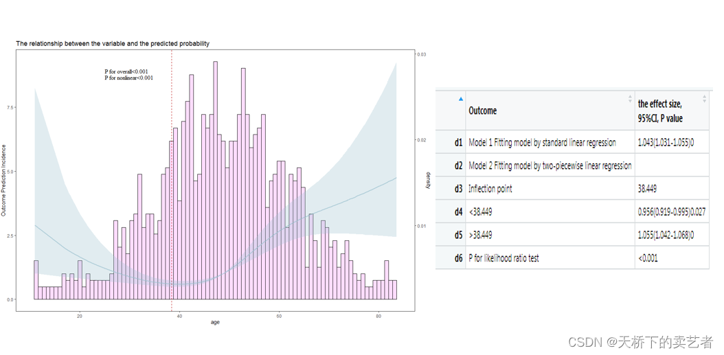
代码+视频，手把手教你R语言ggrcs包绘制限制立方样条图+阈值效应分析_r语言限制立方样条如何找阈值

ggrcs包用于绘制限制立方样条图，目前ggrcs包已经升级到3.5版本了，本人出一个规范的教程和视频，包含有代码，供大家参考。

library(ggrcs)
library(rms)
library(ggplot2)
library(scales)
library(cowplot)

dt<-smoke
dd<-datadist(dt)
options(datadist='dd')
fit<- cph(Surv(time,status==1) ~ rcs(age,4)+gender, x=TRUE, y=TRUE,data=dt)

ggrcs(data=dt,fit=fit,x="age")

#改变柱子颜色
ggrcs(data=dt,fit=fit,x="age",histcol="blue")

#改变柱子宽度，默认是0.8
ggrcs(data=dt,fit=fit,x="age",histcol="blue",histbinwidth=1)

#改变可信区间颜色
ggrcs(data=dt,fit=fit,x="age",histcol="blue",histbinwidth=1,ribcol="green")

#改变可信区间透明度,
ggrcs(data=dt,fit=fit,x="age",histcol="blue",histbinwidth=1,ribcol="green",ribalpha=0.5)

#更改X轴和Y轴和标题内容
ggrcs(data=dt,fit=fit,x="age",histcol="blue",
      histbinwidth=1,ribcol="green",ribalpha=0.5,xlab ="年龄",ylab="吸烟概率",title ="年龄和吸烟概率关系")

#关掉左轴
ggrcs(data=dt,fit=fit,x="age",histcol="blue",
      histbinwidth=1,ribcol="green",ribalpha=0.5,xlab ="年龄",ylab="吸烟概率",
      title ="年龄和吸烟概率关系",lift=F)
#双组
ggrcs(data=dt,fit=fit,x="age",group="gender")

#自定义颜色
ggrcs(data=dt,fit=fit,x="age",group="gender",groupcol=c("red","blue"),histbinwidth=1)

#更改左轴名字
ggrcs(data=dt,fit=fit,x="age",group="gender",
      groupcol=c("red","blue"),histbinwidth=1,ribalpha=0.5,xlab ="年龄",
      ylab="吸烟HR",title ="年龄和吸烟概率关系",liftname="概率密度")

#调整字体位置
ggrcs(data=dt,fit=fit,x="age",group="gender",
      groupcol=c("red","blue"),histbinwidth=1,ribalpha=0.5,xlab ="年龄",
      ylab="吸烟HR",title ="年龄和吸烟概率关系",px=10,py=18)

#风格定制  深海绿+黄金1
ggrcs(data=dt,fit=fit,x="age",group="gender",colset = "A")

###########逻辑回归
library(foreign)
be <- read.spss("E:/r/test/Breast cancer survival agec.sav",
                use.value.labels=F, to.data.frame=T)
be <- na.omit(be)
be$ln_yesno<-as.factor(be$ln_yesno)
dd <- datadist(be) 
options(datadist='dd') 
fit <-lrm(status ~ rcs(age, 4)+ln_yesno,data=be)
ggrcs(data=be,fit=fit,x="age")
ggrcs(data=be,fit=fit,x="age",histbinwidth=1)
ggrcs(data=be,fit=fit,x="age",group="ln_yesno",histbinwidth=1)

##########线性回归
library(foreign)
be <- read.spss("E:/r/test/ozone.sav",
                use.value.labels=F, to.data.frame=T)  #????
be$variables2<-sample(0:1,size=330,replace=TRUE)
be$variables2<-as.factor(be$variables2)
dd <- datadist(be) 
options(datadist='dd') 
fit<-ols(ozon ~rcs(temp, 4)+dpg+variables2,data=be)
ggrcs(data=be,fit=fit,x="temp",histbinwidth=1)
ggrcs(data=be,fit=fit,x="temp",group="variables2",histbinwidth=1)
ggrcs(data=be,fit=fit,x="temp",group="variables2",histbinwidth=1,
      groupcol=c("red","blue"),bordercol="green")

##############singlercs
singlercs(data=dt,fit=fit,x="age")
singlercs(data=dt,fit=fit,x="age",group="gender")

#########
source("E:/r/test/cut.tab1.3.R")
fit<- cph(Surv(time,status==1) ~ rcs(age,4)+gender, x=TRUE, y=TRUE,data=dt)
fit1 <-coxph(Surv(time,status==1) ~ age,data=dt)
out<-cut.tab(fit1,"age",dt)

p<-ggrcs(data=dt,fit=fit,x="age")
p+geom_vline(aes(xintercept=38.449),colour="#BB0000", linetype="dashed")

1
2
3
4
5
6
7
8
9
10
11
12
13
14
15
16
17
18
19
20
21
22
23
24
25
26
27
28
29
30
31
32
33
34
35
36
37
38
39
40
41
42
43
44
45
46
47
48
49
50
51
52
53
54
55
56
57
58
59
60
61
62
63
64
65
66
67
68
69
70
71
72
73
74
75
76
77
78
79
80
81
82
83
84
85
86
87
88
89
90
91
92