
- 1 【全文】狼叔:如何正确的学习Node.js
- 2SpringMVC和Content-Type_mvc content
- 3常见AI模型参数量-以及算力需求评估_小模型算力评估
- 4Spring Boot RestTemplate请求证书问题
- 5配置在关闭本地电脑的情况下远程服务器仍然训练、工作_rdp关闭后保持服务器运行
- 6超融合、软件定义存储(SDS)、分布式存储以及Server SAN的区别与联系_sds存储
- 7linux上网络带宽监控命令,Linux网络带宽监控分析常用命令
- 8html 字体模糊,CSS3 translate导致字体模糊的实例代码
- 9Java 使用过滤器重定向跳转_过滤器重定向到首页
- 10SSM的简单介绍
3D目标检测数据集 KITTI(标签格式解析、3D框可视化、点云转图像、BEV鸟瞰图)
赞
踩
本文介绍在3D目标检测中,理解和使用KITTI 数据集,包括KITTI 的基本情况、下载数据集、标签格式解析、3D框可视化、点云转图像、画BEV鸟瞰图等,并配有实现代码。
目录
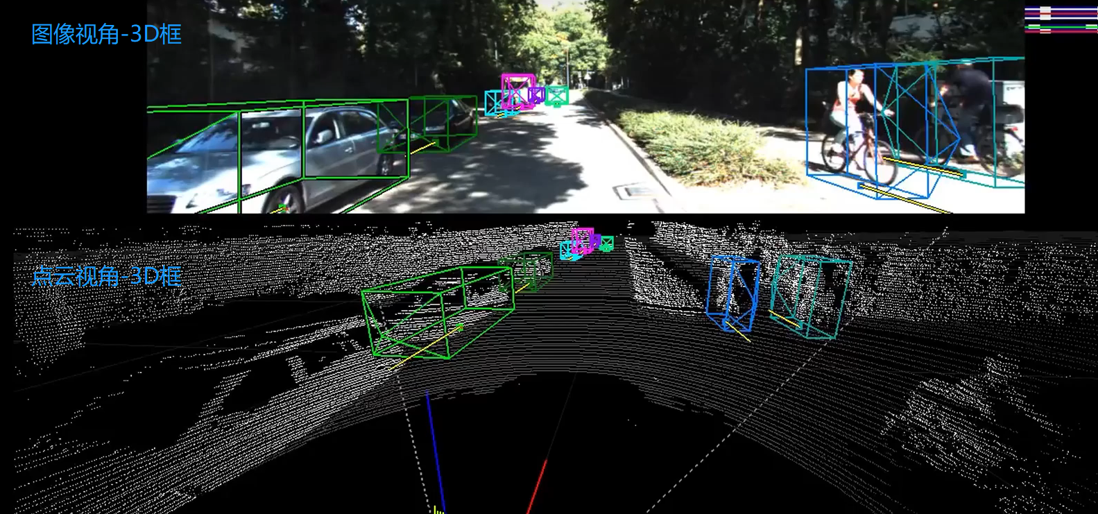
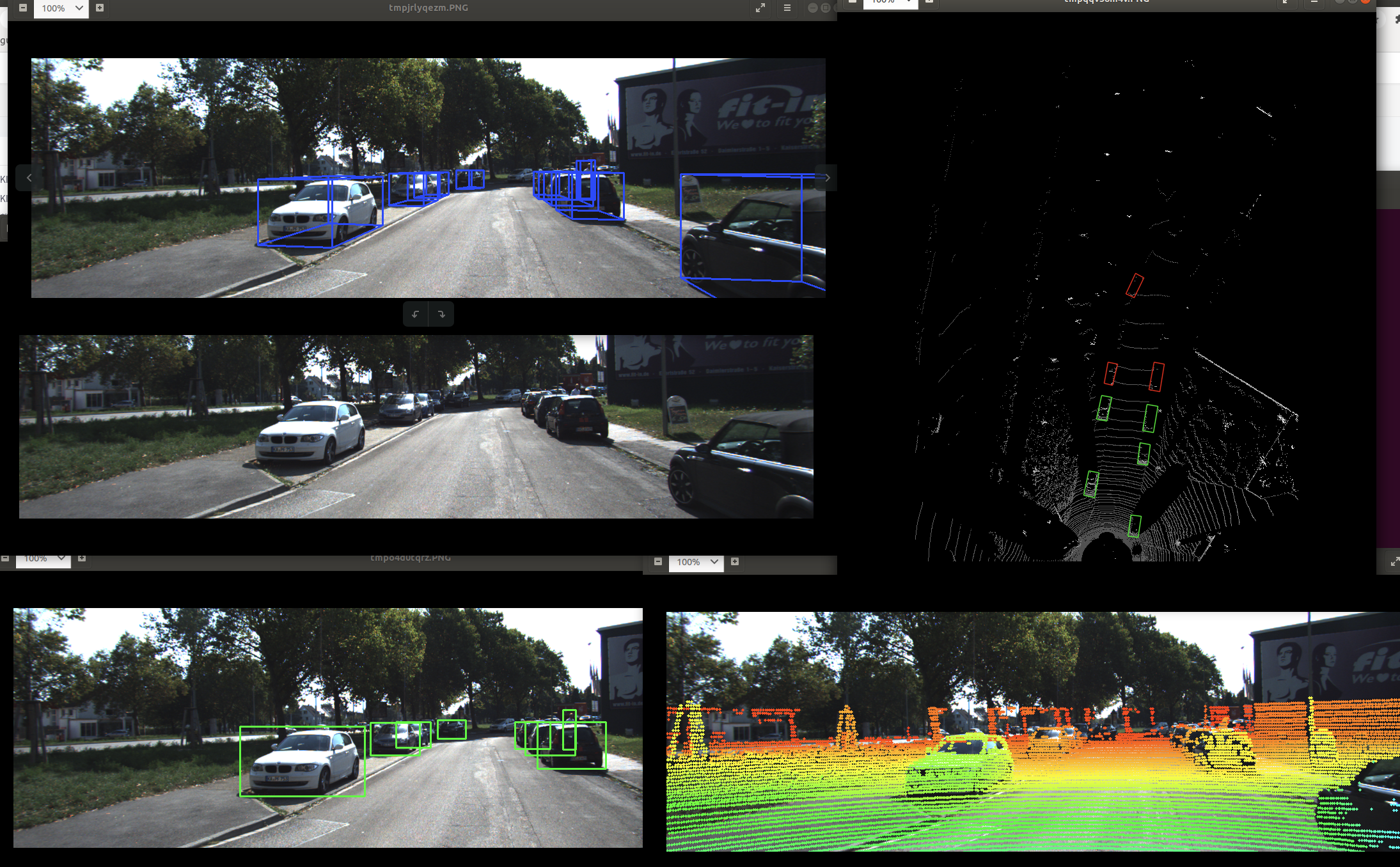
1、KITTI数据集3D框可视化
2、KITTI 3D数据集
kitti 3D数据集的基本情况:

KITTI整个数据集是在德国卡尔斯鲁厄采集的,采集时长6小时。KITTI官网放出的数据大约占采集全部的25%,去除了测试集中相关的数据片段,按场景可以分为“道路”、“城市”、“住宅区”、“校园”和“行人”5类。
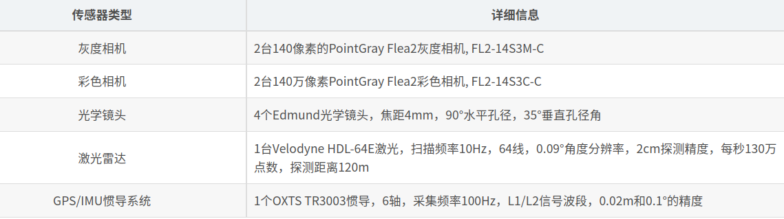
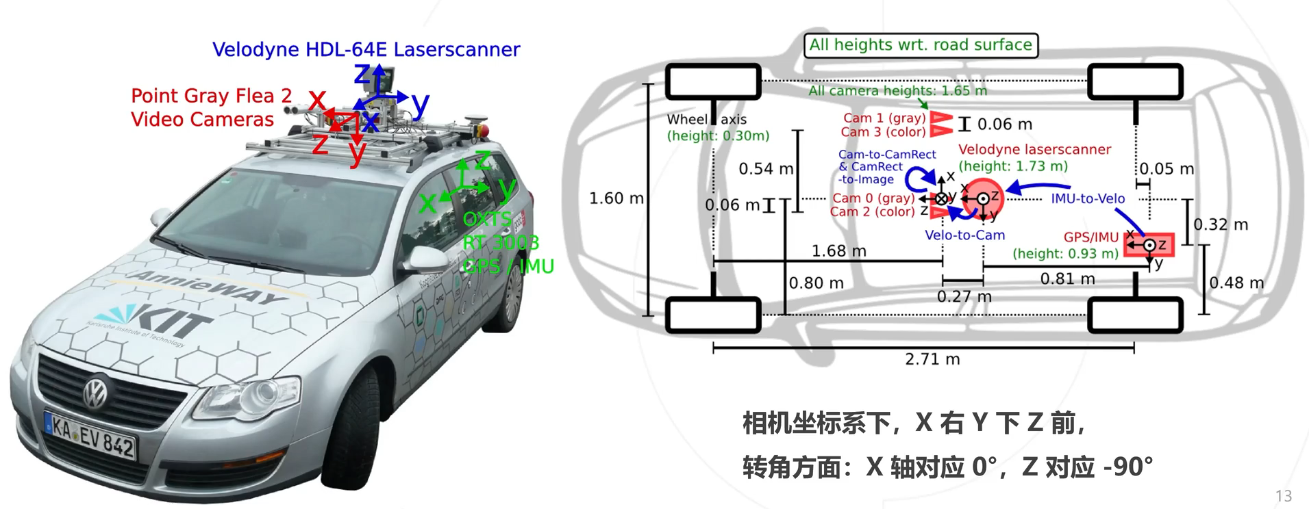
传感器配置:
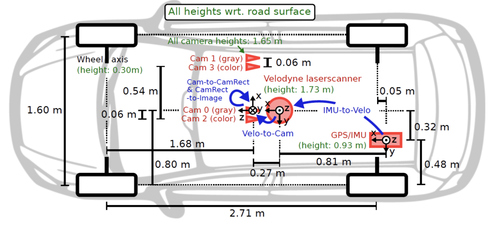
传感器安装位置:
3、下载数据集
The KITTI Vision Benchmark Suite (cvlibs.net)

下载数据需要注册账号的,获取取百度网盘下载;文件的格式如下所示
图片格式:xxx.jpg
点云格式:xxx.bin(点云是以bin二进制的方式存储的)
标定参数:xxx.txt(一个文件中包括各个相机的内参、畸变校正矩阵、激光雷达坐标转到相机坐标的矩阵、IMU坐标转到激光雷达坐标的矩阵)
标签格式:xxx.txt(包含类别、截断情况、遮挡情况、观测角度、2D框左上角坐标、2D框右下角坐标、3D物体的尺寸-高宽长、3D物体的中心坐标-xyz、置信度)
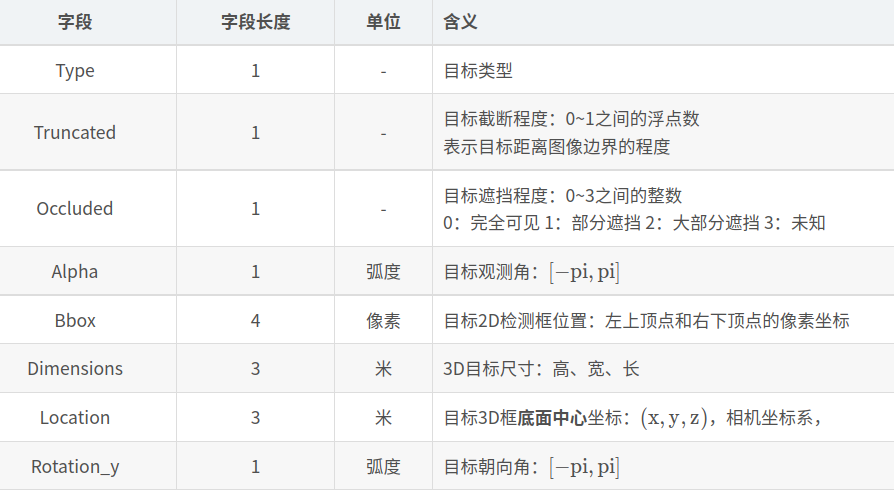
4、标签格式
示例标签:Pedestrian 0.00 0 -0.20 712.40 143.00 810.73 307.92 1.89 0.48 1.20 1.84 1.47 8.41 0.01

这时可以看看这个视频:
5、标定参数解析
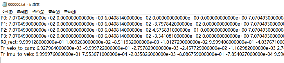
然后看一下标定参数:
P0-P3:是各个相机的内参矩阵;3×4的相机投影矩阵,0~3分别对应左侧灰度相机、右侧灰度相机、左侧彩色相机、右侧彩色相机。
R0_rect: 是左相机的畸变矫正矩阵;3×3的旋转修正矩阵。
Tr_velo_to_cam:是激光雷达坐标系 转到 相机坐标系矩阵;3×4的激光坐标系到Cam 0坐标系的变换矩阵。
Tr_imu_to_velo: 是IMU坐标转到激光雷达坐标的矩阵;3×4的IMU坐标系到激光坐标系的变换矩阵。
6、点云数据-->投影到图像
当有了点云数据信息,如何投影到图像中呢?本质上是一个坐标系转换的问题,流程思路如下:
- 已知点云坐标(x,y,z),当前是处于激光雷达坐标系
- 激光雷达坐标系 转到 相机坐标系,需要用到标定参数中的Tr_velo_to_cam矩阵,此时得到相机坐标(x1,y1,z1)
- 相机坐标系进行畸变矫正,需要用到标定参数中的R0_rect矩阵,此时得到相机坐标(x2,y2,z2)
- 相机坐标系转为图像坐标系,需要用到标定参数中的P0矩阵,即相机内存矩阵,此时得到图像坐标(u,v)
看一下示例效果:

接口代码:
- '''
- 将点云数据投影到图像
- '''
- def show_lidar_on_image(pc_velo, img, calib, img_width, img_height):
- ''' Project LiDAR points to image '''
- imgfov_pc_velo, pts_2d, fov_inds = get_lidar_in_image_fov(pc_velo,
- calib, 0, 0, img_width, img_height, True)
- imgfov_pts_2d = pts_2d[fov_inds,:]
- imgfov_pc_rect = calib.project_velo_to_rect(imgfov_pc_velo)
-
- import matplotlib.pyplot as plt
- cmap = plt.cm.get_cmap('hsv', 256)
- cmap = np.array([cmap(i) for i in range(256)])[:,:3]*255
-
- for i in range(imgfov_pts_2d.shape[0]):
- depth = imgfov_pc_rect[i,2]
- color = cmap[int(640.0/depth),:]
- cv2.circle(img, (int(np.round(imgfov_pts_2d[i,0])),
- int(np.round(imgfov_pts_2d[i,1]))),
- 2, color=tuple(color), thickness=-1)
- Image.fromarray(img).save('save_output/lidar_on_image.png')
- Image.fromarray(img).show()
- return img

核心代码:
- '''
- 将点云数据投影到相机坐标系
- '''
- def get_lidar_in_image_fov(pc_velo, calib, xmin, ymin, xmax, ymax,
- return_more=False, clip_distance=2.0):
- ''' Filter lidar points, keep those in image FOV '''
- pts_2d = calib.project_velo_to_image(pc_velo)
- fov_inds = (pts_2d[:,0]<xmax) & (pts_2d[:,0]>=xmin) & \
- (pts_2d[:,1]<ymax) & (pts_2d[:,1]>=ymin)
- fov_inds = fov_inds & (pc_velo[:,0]>clip_distance)
- imgfov_pc_velo = pc_velo[fov_inds,:]
- if return_more:
- return imgfov_pc_velo, pts_2d, fov_inds
- else:
- return imgfov_pc_velo
7、图像数据-->投影到点云
当有了图像RGB信息,如何投影到点云中呢?本质上是一个坐标系转换的问题,和上面的是逆过程,流程思路如下:
- 已知图像坐标(u,v),当前是处于图像坐标系
- 图像坐标系 转 相机坐标系,需要用到标定参数中的P0逆矩阵,即相机内存矩阵,得到相机坐标(x,y,z)
- 相机坐标系进行畸变矫正,需要用到标定参数中的R0_rect逆矩阵,得到相机坐标(x1,y1,z1)
- 矫正后相机坐标系 转 激光雷达坐标系,需要用到标定参数中的Tr_velo_to_cam逆矩阵,此时得到激光雷达坐标(x2,y2,z2)
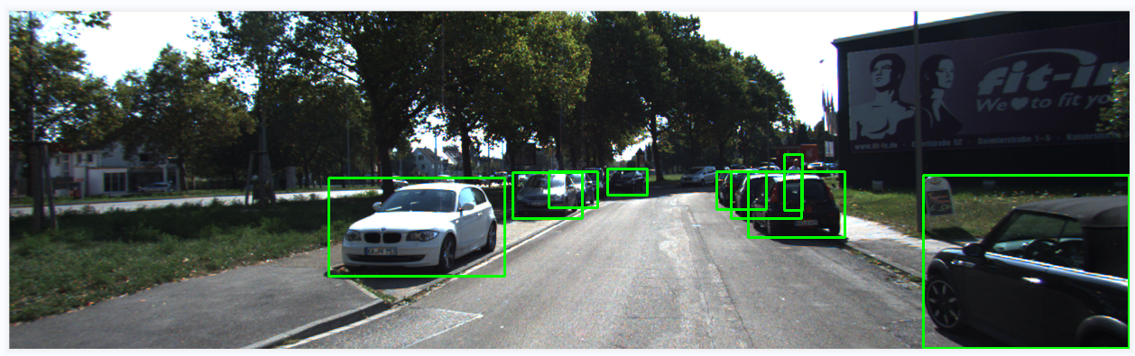
8、可视化图像2D结果、3D结果
先看一下2D框的效果:
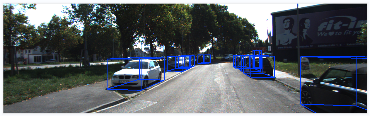
3D框的效果:
接口代码:
- '''
- 在图像中画2D框、3D框
- '''
- def show_image_with_boxes(img, objects, calib, show3d=True):
- img1 = np.copy(img) # for 2d bbox
- img2 = np.copy(img) # for 3d bbox
- for obj in objects:
- if obj.type=='DontCare':continue
- cv2.rectangle(img1, (int(obj.xmin),int(obj.ymin)), (int(obj.xmax),int(obj.ymax)), (0,255,0), 2) # 画2D框
- box3d_pts_2d, box3d_pts_3d = utils.compute_box_3d(obj, calib.P) # 获取图像3D框(8*2)、相机坐标系3D框(8*3)
- img2 = utils.draw_projected_box3d(img2, box3d_pts_2d) # 在图像上画3D框
- if show3d:
- Image.fromarray(img2).save('save_output/image_with_3Dboxes.png')
- Image.fromarray(img2).show()
- else:
- Image.fromarray(img1).save('save_output/image_with_2Dboxes.png')
- Image.fromarray(img1).show()
核心代码:
- def compute_box_3d(obj, P):
- '''
- 计算对象的3D边界框在图像平面上的投影
- 输入: obj代表一个物体标签信息, P代表相机的投影矩阵-内参。
- 输出: 返回两个值, corners_3d表示3D边界框在 相机坐标系 的8个角点的坐标-3D坐标。
- corners_2d表示3D边界框在 图像上 的8个角点的坐标-2D坐标。
- '''
- # 计算一个绕Y轴旋转的旋转矩阵R,用于将3D坐标从世界坐标系转换到相机坐标系。obj.ry是对象的偏航角
- R = roty(obj.ry)
-
- # 物体实际的长、宽、高
- l = obj.l;
- w = obj.w;
- h = obj.h;
-
- # 存储了3D边界框的8个角点相对于对象中心的坐标。这些坐标定义了3D边界框的形状。
- x_corners = [l/2,l/2,-l/2,-l/2,l/2,l/2,-l/2,-l/2];
- y_corners = [0,0,0,0,-h,-h,-h,-h];
- z_corners = [w/2,-w/2,-w/2,w/2,w/2,-w/2,-w/2,w/2];
-
- # 1、将3D边界框的角点坐标从对象坐标系转换到相机坐标系。它使用了旋转矩阵R
- corners_3d = np.dot(R, np.vstack([x_corners,y_corners,z_corners]))
- # 3D边界框的坐标进行平移
- corners_3d[0,:] = corners_3d[0,:] + obj.t[0];
- corners_3d[1,:] = corners_3d[1,:] + obj.t[1];
- corners_3d[2,:] = corners_3d[2,:] + obj.t[2];
-
- # 2、检查对象是否在相机前方,因为只有在相机前方的对象才会被绘制。
- # 如果对象的Z坐标(深度)小于0.1,就意味着对象在相机后方,那么corners_2d将被设置为None,函数将返回None。
- if np.any(corners_3d[2,:]<0.1):
- corners_2d = None
- return corners_2d, np.transpose(corners_3d)
-
- # 3、将相机坐标系下的3D边界框的角点,投影到图像平面上,得到它们在图像上的2D坐标。
- corners_2d = project_to_image(np.transpose(corners_3d), P);
- return corners_2d, np.transpose(corners_3d)
-
-
- def draw_projected_box3d(image, qs, color=(0,60,255), thickness=2):
- '''
- qs: 包含8个3D边界框角点坐标的数组, 形状为(8, 2)。图像坐标下的3D框, 8个顶点坐标。
- '''
- ''' Draw 3d bounding box in image
- qs: (8,2) array of vertices for the 3d box in following order:
- 1 -------- 0
- /| /|
- 2 -------- 3 .
- | | | |
- . 5 -------- 4
- |/ |/
- 6 -------- 7
- '''
- qs = qs.astype(np.int32) # 将输入的顶点坐标转换为整数类型,以便在图像上绘制。
-
- # 这个循环迭代4次,每次处理一个边界框的一条边。
- for k in range(0,4):
- # Ref: http://docs.enthought.com/mayavi/mayavi/auto/mlab_helper_functions.html
-
- # 定义了要绘制的边的起始点和结束点的索引。在这个循环中,它用于绘制边界框的前四条边。
- i,j=k,(k+1)%4
- cv2.line(image, (qs[i,0],qs[i,1]), (qs[j,0],qs[j,1]), color, thickness)
-
- # 定义了要绘制的边的起始点和结束点的索引。在这个循环中,它用于绘制边界框的后四条边,与前四条边平行
- i,j=k+4,(k+1)%4 + 4
- cv2.line(image, (qs[i,0],qs[i,1]), (qs[j,0],qs[j,1]), color, thickness)
-
- # 定义了要绘制的边的起始点和结束点的索引。在这个循环中,它用于绘制连接前四条边和后四条边的边界框的边。
- i,j=k,k+4
- cv2.line(image, (qs[i,0],qs[i,1]), (qs[j,0],qs[j,1]), color, thickness)
- return image
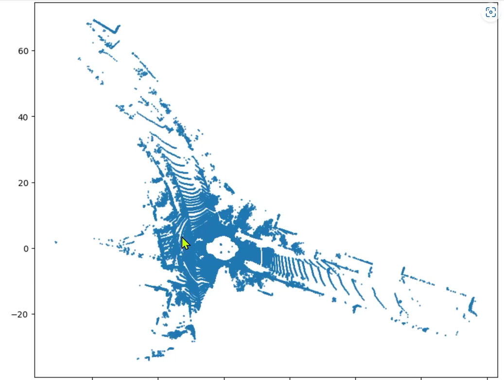
9、点云3D结果-->图像BEV鸟瞰图结果(坐标系转换)
思路流程:
- 读取点云数据,点云得存储格式是n*4,n是指当前文件点云的数量,4分别表示(x,y,z,intensity),即点云的空间三维坐标、反射强度
- 我们只需读取前两行即可,得到坐标点(x,y)
- 然后将坐标点(x,y),画散点图
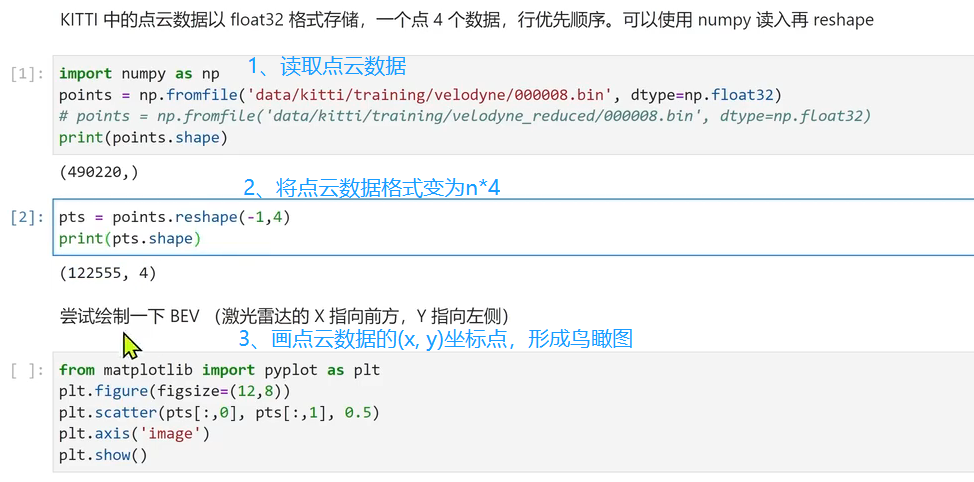
BEV鸟瞰图效果如下:
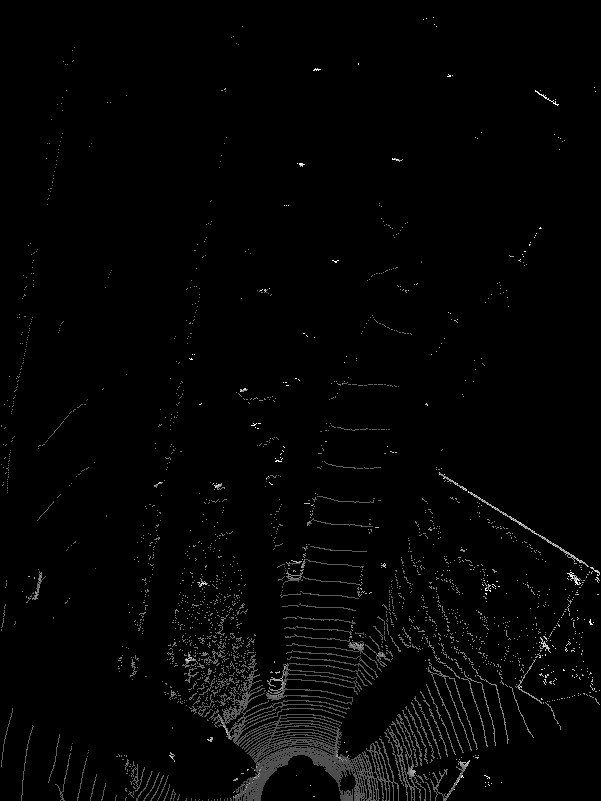
10、绘制BEV鸟瞰图
BEV图像示例效果:
核心代码:
-
- '''
- 可视化BEV鸟瞰图
- '''
- def show_lidar_topview(pc_velo, objects, calib):
- # 1-设置鸟瞰图范围
- side_range = (-30, 30) # 左右距离
- fwd_range = (0, 80) # 后前距离
-
- x_points = pc_velo[:, 0]
- y_points = pc_velo[:, 1]
- z_points = pc_velo[:, 2]
-
- # 2-获得区域内的点
- f_filt = np.logical_and(x_points > fwd_range[0], x_points < fwd_range[1])
- s_filt = np.logical_and(y_points > side_range[0], y_points < side_range[1])
- filter = np.logical_and(f_filt, s_filt)
- indices = np.argwhere(filter).flatten()
- x_points = x_points[indices]
- y_points = y_points[indices]
- z_points = z_points[indices]
-
- # 定义了鸟瞰图中每个像素代表的距离
- res = 0.1
- # 3-1将点云坐标系 转到 BEV坐标系
- x_img = (-y_points / res).astype(np.int32)
- y_img = (-x_points / res).astype(np.int32)
- # 3-2调整坐标原点
- x_img -= int(np.floor(side_range[0]) / res)
- y_img += int(np.floor(fwd_range[1]) / res)
- print(x_img.min(), x_img.max(), y_img.min(), y_img.max())
-
- # 4-填充像素值, 将点云数据的高度信息(Z坐标)映射到像素值
- height_range = (-3, 1.0)
- pixel_value = np.clip(a=z_points, a_max=height_range[1], a_min=height_range[0])
-
-
- def scale_to_255(a, min, max, dtype=np.uint8):
- return ((a - min) / float(max - min) * 255).astype(dtype)
-
- pixel_value = scale_to_255(pixel_value, height_range[0], height_range[1])
-
- # 创建图像数组
- x_max = 1 + int((side_range[1] - side_range[0]) / res)
- y_max = 1 + int((fwd_range[1] - fwd_range[0]) / res)
- im = np.zeros([y_max, x_max], dtype=np.uint8)
- im[y_img, x_img] = pixel_value
-
- im2 = Image.fromarray(im)
- im2.save('save_output/BEV.png')
- im2.show()
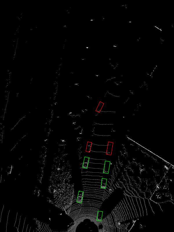
11、BEV鸟瞰图画2d框
在BEV视图中画框,可视化结果:
接口代码:
- '''
- 将点云数据3D框投影到BEV
- '''
- def show_lidar_topview_with_boxes(img, objects, calib):
- def bbox3d(obj):
- box3d_pts_2d, box3d_pts_3d = utils.compute_box_3d(obj, calib.P) # 获取3D框-图像、3D框-相机坐标系
- box3d_pts_3d_velo = calib.project_rect_to_velo(box3d_pts_3d) # 将相机坐标系的框 转到 激光雷达坐标系
- return box3d_pts_3d_velo # 返回nx3的点
-
- boxes3d = [bbox3d(obj) for obj in objects if obj.type == "Car"]
- gt = np.array(boxes3d)
- im2 = utils.draw_box3d_label_on_bev(img, gt, scores=None, thickness=1) # 获取激光雷达坐标系的3D点,选择x, y两维,画到BEV平面坐标系上
- im2 = Image.fromarray(im2)
- im2.save('save_output/BEV with boxes.png')
- im2.show()
核心代码:
- # 设置BEV鸟瞰图参数
- side_range = (-30, 30) # 左右距离
- fwd_range = (0, 80) # 后前距离
- res = 0.1 # 分辨率0.05m
-
- def compute_box_3d(obj, P):
- '''
- 计算对象的3D边界框在图像平面上的投影
- 输入: obj代表一个物体标签信息, P代表相机的投影矩阵-内参。
- 输出: 返回两个值, corners_3d表示3D边界框在 相机坐标系 的8个角点的坐标-3D坐标。
- corners_2d表示3D边界框在 图像上 的8个角点的坐标-2D坐标。
- '''
- # 计算一个绕Y轴旋转的旋转矩阵R,用于将3D坐标从世界坐标系转换到相机坐标系。obj.ry是对象的偏航角
- R = roty(obj.ry)
-
- # 物体实际的长、宽、高
- l = obj.l;
- w = obj.w;
- h = obj.h;
-
- # 存储了3D边界框的8个角点相对于对象中心的坐标。这些坐标定义了3D边界框的形状。
- x_corners = [l/2,l/2,-l/2,-l/2,l/2,l/2,-l/2,-l/2];
- y_corners = [0,0,0,0,-h,-h,-h,-h];
- z_corners = [w/2,-w/2,-w/2,w/2,w/2,-w/2,-w/2,w/2];
-
- # 1、将3D边界框的角点坐标从对象坐标系转换到相机坐标系。它使用了旋转矩阵R
- corners_3d = np.dot(R, np.vstack([x_corners,y_corners,z_corners]))
- # 3D边界框的坐标进行平移
- corners_3d[0,:] = corners_3d[0,:] + obj.t[0];
- corners_3d[1,:] = corners_3d[1,:] + obj.t[1];
- corners_3d[2,:] = corners_3d[2,:] + obj.t[2];
-
- # 2、检查对象是否在相机前方,因为只有在相机前方的对象才会被绘制。
- # 如果对象的Z坐标(深度)小于0.1,就意味着对象在相机后方,那么corners_2d将被设置为None,函数将返回None。
- if np.any(corners_3d[2,:]<0.1):
- corners_2d = None
- return corners_2d, np.transpose(corners_3d)
-
- # 3、将相机坐标系下的3D边界框的角点,投影到图像平面上,得到它们在图像上的2D坐标。
- corners_2d = project_to_image(np.transpose(corners_3d), P);
- return corners_2d, np.transpose(corners_3d)
-
-
-
12、完整工程代码
工程目录:

kitti_vis_main.py(主代码入口)
-
- from __future__ import print_function
-
- import os
- import sys
- import cv2
- import os.path
- from PIL import Image
- BASE_DIR = os.path.dirname(os.path.abspath(__file__))
- ROOT_DIR = os.path.dirname(BASE_DIR)
- sys.path.append(BASE_DIR)
- sys.path.append(os.path.join(ROOT_DIR, 'mayavi'))
- from kitti_object import *
-
-
- def visualization():
- import mayavi.mlab as mlab
- dataset = kitti_object(os.path.join(ROOT_DIR, 'Kitti_3D_Vis/dataset/object')) # linux 路径
- data_idx = 10 # 选择第几张图像
-
- # 1-加载标签数据
- objects = dataset.get_label_objects(data_idx)
- print("There are %d objects.", len(objects))
-
- # 2-加载图像
- img = dataset.get_image(data_idx)
- img = cv2.cvtColor(img, cv2.COLOR_BGR2RGB)
- img_height, img_width, img_channel = img.shape
-
- # 3-加载点云数据
- pc_velo = dataset.get_lidar(data_idx)[:,0:3] # (x, y, z)
-
- # 4-加载标定参数
- calib = dataset.get_calibration(data_idx)
-
- # 5-可视化原始图像
- print(' ------------ show raw image -------- ')
- Image.fromarray(img).show()
-
- # 6-在图像中画2D框
- print(' ------------ show image with 2D bounding box -------- ')
- show_image_with_boxes(img, objects, calib, False)
-
- # 7-在图像中画3D框
- print(' ------------ show image with 3D bounding box ------- ')
- show_image_with_boxes(img, objects, calib, True)
-
- # 8-将点云数据投影到图像
- print(' ----------- LiDAR points projected to image plane -- ')
- show_lidar_on_image(pc_velo, img, calib, img_width, img_height)
-
- # 9-画BEV图
- print('------------------ BEV of LiDAR points -----------------------------')
- show_lidar_topview(pc_velo, objects, calib)
-
- # 10-在BEV图中画2D框
- print('--------------- BEV of LiDAR points with bobes ---------------------')
- img1 = cv2.imread('save_output/BEV.png')
- img = cv2.cvtColor(img1, cv2.COLOR_BGR2RGB)
- show_lidar_topview_with_boxes(img1, objects, calib)
-
-
- if __name__=='__main__':
- visualization()
kitti_util.py
- from __future__ import print_function
-
- import numpy as np
- import cv2
- from PIL import Image
- import os
-
- # 设置BEV鸟瞰图参数
- side_range = (-30, 30) # 左右距离
- fwd_range = (0, 80) # 后前距离
- res = 0.1 # 分辨率0.05m
-
- def compute_box_3d(obj, P):
- '''
- 计算对象的3D边界框在图像平面上的投影
- 输入: obj代表一个物体标签信息, P代表相机的投影矩阵-内参。
- 输出: 返回两个值, corners_3d表示3D边界框在 相机坐标系 的8个角点的坐标-3D坐标。
- corners_2d表示3D边界框在 图像上 的8个角点的坐标-2D坐标。
- '''
- # 计算一个绕Y轴旋转的旋转矩阵R,用于将3D坐标从世界坐标系转换到相机坐标系。obj.ry是对象的偏航角
- R = roty(obj.ry)
-
- # 物体实际的长、宽、高
- l = obj.l;
- w = obj.w;
- h = obj.h;
-
- # 存储了3D边界框的8个角点相对于对象中心的坐标。这些坐标定义了3D边界框的形状。
- x_corners = [l/2,l/2,-l/2,-l/2,l/2,l/2,-l/2,-l/2];
- y_corners = [0,0,0,0,-h,-h,-h,-h];
- z_corners = [w/2,-w/2,-w/2,w/2,w/2,-w/2,-w/2,w/2];
-
- # 1、将3D边界框的角点坐标从对象坐标系转换到相机坐标系。它使用了旋转矩阵R
- corners_3d = np.dot(R, np.vstack([x_corners,y_corners,z_corners]))
- # 3D边界框的坐标进行平移
- corners_3d[0,:] = corners_3d[0,:] + obj.t[0];
- corners_3d[1,:] = corners_3d[1,:] + obj.t[1];
- corners_3d[2,:] = corners_3d[2,:] + obj.t[2];
-
- # 2、检查对象是否在相机前方,因为只有在相机前方的对象才会被绘制。
- # 如果对象的Z坐标(深度)小于0.1,就意味着对象在相机后方,那么corners_2d将被设置为None,函数将返回None。
- if np.any(corners_3d[2,:]<0.1):
- corners_2d = None
- return corners_2d, np.transpose(corners_3d)
-
- # 3、将相机坐标系下的3D边界框的角点,投影到图像平面上,得到它们在图像上的2D坐标。
- corners_2d = project_to_image(np.transpose(corners_3d), P);
- return corners_2d, np.transpose(corners_3d)
-
-
- def project_to_image(pts_3d, P):
- '''
- 将相机坐标系下的3D边界框的角点, 投影到图像平面上, 得到它们在图像上的2D坐标
- 输入: pts_3d是一个nx3的矩阵, 包含了待投影的3D坐标点(每行一个点), P是相机的投影矩阵, 通常是一个3x4的矩阵。
- 输出: 返回一个nx2的矩阵, 包含了投影到图像平面上的2D坐标点。
- P(3x4) dot pts_3d_extended(4xn) = projected_pts_2d(3xn) => normalize projected_pts_2d(2xn)
- <=> pts_3d_extended(nx4) dot P'(4x3) = projected_pts_2d(nx3) => normalize projected_pts_2d(nx2)
- '''
- n = pts_3d.shape[0] # 获取3D点的数量
- pts_3d_extend = np.hstack((pts_3d, np.ones((n,1)))) # 将每个3D点的坐标扩展为齐次坐标形式(4D),通过在每个点的末尾添加1,创建了一个nx4的矩阵。
- pts_2d = np.dot(pts_3d_extend, np.transpose(P)) # 将扩展的3D坐标点矩阵与投影矩阵P相乘,得到一个nx3的矩阵,其中每一行包含了3D点在图像平面上的投影坐标。每个点的坐标表示为[x, y, z]。
- pts_2d[:,0] /= pts_2d[:,2] # 将投影坐标中的x坐标除以z坐标,从而获得2D图像上的x坐标。
- pts_2d[:,1] /= pts_2d[:,2] # 将投影坐标中的y坐标除以z坐标,从而获得2D图像上的y坐标。
- return pts_2d[:,0:2] # 返回一个nx2的矩阵,其中包含了每个3D点在2D图像上的坐标。
-
-
-
- def draw_projected_box3d(image, qs, color=(0,60,255), thickness=2):
- '''
- qs: 包含8个3D边界框角点坐标的数组, 形状为(8, 2)。图像坐标下的3D框, 8个顶点坐标。
- '''
- ''' Draw 3d bounding box in image
- qs: (8,2) array of vertices for the 3d box in following order:
- 1 -------- 0
- /| /|
- 2 -------- 3 .
- | | | |
- . 5 -------- 4
- |/ |/
- 6 -------- 7
- '''
- qs = qs.astype(np.int32) # 将输入的顶点坐标转换为整数类型,以便在图像上绘制。
-
- # 这个循环迭代4次,每次处理一个边界框的一条边。
- for k in range(0,4):
- # Ref: http://docs.enthought.com/mayavi/mayavi/auto/mlab_helper_functions.html
-
- # 定义了要绘制的边的起始点和结束点的索引。在这个循环中,它用于绘制边界框的前四条边。
- i,j=k,(k+1)%4
- cv2.line(image, (qs[i,0],qs[i,1]), (qs[j,0],qs[j,1]), color, thickness)
-
- # 定义了要绘制的边的起始点和结束点的索引。在这个循环中,它用于绘制边界框的后四条边,与前四条边平行
- i,j=k+4,(k+1)%4 + 4
- cv2.line(image, (qs[i,0],qs[i,1]), (qs[j,0],qs[j,1]), color, thickness)
-
- # 定义了要绘制的边的起始点和结束点的索引。在这个循环中,它用于绘制连接前四条边和后四条边的边界框的边。
- i,j=k,k+4
- cv2.line(image, (qs[i,0],qs[i,1]), (qs[j,0],qs[j,1]), color, thickness)
- return image
-
- def draw_box3d_label_on_bev(image, boxes3d, thickness=1, scores=None):
- # if scores is not None and scores.shape[0] >0:
- img = image.copy()
- num = len(boxes3d)
- for n in range(num):
- b = boxes3d[n]
- x0 = b[0, 0]
- y0 = b[0, 1]
- x1 = b[1, 0]
- y1 = b[1, 1]
- x2 = b[2, 0]
- y2 = b[2, 1]
- x3 = b[3, 0]
- y3 = b[3, 1]
- if (x0<30 and x1<30 and x2<30 and x3<30):
- u0, v0 = lidar_to_top_coords(x0, y0)
- u1, v1 = lidar_to_top_coords(x1, y1)
- u2, v2 = lidar_to_top_coords(x2, y2)
- u3, v3 = lidar_to_top_coords(x3, y3)
- color = (0, 255, 0) # green
- cv2.line(img, (u0, v0), (u1, v1), color, thickness, cv2.LINE_AA)
- cv2.line(img, (u1, v1), (u2, v2), color, thickness, cv2.LINE_AA)
- cv2.line(img, (u2, v2), (u3, v3), color, thickness, cv2.LINE_AA)
- cv2.line(img, (u3, v3), (u0, v0), color, thickness, cv2.LINE_AA)
- elif (x0<50 and x1<50 and x2<50 and x3<50):
- color = (255, 0, 0) # red
- u0, v0 = lidar_to_top_coords(x0, y0)
- u1, v1 = lidar_to_top_coords(x1, y1)
- u2, v2 = lidar_to_top_coords(x2, y2)
- u3, v3 = lidar_to_top_coords(x3, y3)
- cv2.line(img, (u0, v0), (u1, v1), color, thickness, cv2.LINE_AA)
- cv2.line(img, (u1, v1), (u2, v2), color, thickness, cv2.LINE_AA)
- cv2.line(img, (u2, v2), (u3, v3), color, thickness, cv2.LINE_AA)
- cv2.line(img, (u3, v3), (u0, v0), color, thickness, cv2.LINE_AA)
- else:
- color = (0, 0, 255) # blue
- u0, v0 = lidar_to_top_coords(x0, y0)
- u1, v1 = lidar_to_top_coords(x1, y1)
- u2, v2 = lidar_to_top_coords(x2, y2)
- u3, v3 = lidar_to_top_coords(x3, y3)
- cv2.line(img, (u0, v0), (u1, v1), color, thickness, cv2.LINE_AA)
- cv2.line(img, (u1, v1), (u2, v2), color, thickness, cv2.LINE_AA)
- cv2.line(img, (u2, v2), (u3, v3), color, thickness, cv2.LINE_AA)
- cv2.line(img, (u3, v3), (u0, v0), color, thickness, cv2.LINE_AA)
-
- return img
-
- def draw_box3d_predict_on_bev(image, boxes3d, thickness=1, scores=None):
- # if scores is not None and scores.shape[0] >0:
- img = image.copy()
- num = len(boxes3d)
- for n in range(num):
- b = boxes3d[n]
- x0 = b[0, 0]
- y0 = b[0, 1]
- x1 = b[1, 0]
- y1 = b[1, 1]
- x2 = b[2, 0]
- y2 = b[2, 1]
- x3 = b[3, 0]
- y3 = b[3, 1]
- color = (255, 255, 255) # white
- u0, v0 = lidar_to_top_coords(x0, y0)
- u1, v1 = lidar_to_top_coords(x1, y1)
- u2, v2 = lidar_to_top_coords(x2, y2)
- u3, v3 = lidar_to_top_coords(x3, y3)
- cv2.line(img, (u0, v0), (u1, v1), color, thickness, cv2.LINE_AA)
- cv2.line(img, (u1, v1), (u2, v2), color, thickness, cv2.LINE_AA)
- cv2.line(img, (u2, v2), (u3, v3), color, thickness, cv2.LINE_AA)
- cv2.line(img, (u3, v3), (u0, v0), color, thickness, cv2.LINE_AA)
- return img
-
- def lidar_to_top_coords(x, y, z=None):
- if 0:
- return x, y
- else:
- # print("TOP_X_MAX-TOP_X_MIN:",TOP_X_MAX,TOP_X_MIN)
- xx = (-y / res).astype(np.int32)
- yy = (-x / res).astype(np.int32)
- # 调整坐标原点
- xx -= int(np.floor(side_range[0]) / res)
- yy += int(np.floor(fwd_range[1]) / res)
- return xx, yy
-
-
- # 解析标签数据
- class Object3d(object):
- ''' 3d object label '''
- def __init__(self, label_file_line):
- data = label_file_line.split(' ')
- data[1:] = [float(x) for x in data[1:]]
-
- # extract label, truncation, occlusion
- self.type = data[0] # 'Car', 'Pedestrian', ...
- self.truncation = data[1] # truncated pixel ratio [0..1]
- self.occlusion = int(data[2]) # 0=visible, 1=partly occluded, 2=fully occluded, 3=unknown
- self.alpha = data[3] # object observation angle [-pi..pi]
-
- # extract 2d bounding box in 0-based coordinates
- self.xmin = data[4] # left
- self.ymin = data[5] # top
- self.xmax = data[6] # right
- self.ymax = data[7] # bottom
- self.box2d = np.array([self.xmin,self.ymin,self.xmax,self.ymax])
-
- # extract 3d bounding box information
- self.h = data[8] # box height
- self.w = data[9] # box width
- self.l = data[10] # box length (in meters)
- self.t = (data[11],data[12],data[13]) # location (x,y,z) in camera coord.
- self.ry = data[14] # yaw angle (around Y-axis in camera coordinates) [-pi..pi]
-
- def print_object(self):
- print('Type, truncation, occlusion, alpha: %s, %d, %d, %f' % \
- (self.type, self.truncation, self.occlusion, self.alpha))
- print('2d bbox (x0,y0,x1,y1): %f, %f, %f, %f' % \
- (self.xmin, self.ymin, self.xmax, self.ymax))
- print('3d bbox h,w,l: %f, %f, %f' % \
- (self.h, self.w, self.l))
- print('3d bbox location, ry: (%f, %f, %f), %f' % \
- (self.t[0],self.t[1],self.t[2],self.ry))
-
-
- class Calibration(object):
- ''' Calibration matrices and utils
- 3d XYZ in <label>.txt are in rect camera coord.
- 2d box xy are in image2 coord
- Points in <lidar>.bin are in Velodyne coord.
- y_image2 = P^2_rect * x_rect
- y_image2 = P^2_rect * R0_rect * Tr_velo_to_cam * x_velo
- x_ref = Tr_velo_to_cam * x_velo
- x_rect = R0_rect * x_ref
- P^2_rect = [f^2_u, 0, c^2_u, -f^2_u b^2_x;
- 0, f^2_v, c^2_v, -f^2_v b^2_y;
- 0, 0, 1, 0]
- = K * [1|t]
- image2 coord:
- ----> x-axis (u)
- |
- |
- v y-axis (v)
- velodyne coord:
- front x, left y, up z
- rect/ref camera coord:
- right x, down y, front z
- Ref (KITTI paper): http://www.cvlibs.net/publications/Geiger2013IJRR.pdf
- TODO(rqi): do matrix multiplication only once for each projection.
- '''
- def __init__(self, calib_filepath, from_video=False):
- if from_video:
- calibs = self.read_calib_from_video(calib_filepath)
- else:
- calibs = self.read_calib_file(calib_filepath)
- # Projection matrix from rect camera coord to image2 coord
- self.P = calibs['P2']
- self.P = np.reshape(self.P, [3,4])
- # Rigid transform from Velodyne coord to reference camera coord
- self.V2C = calibs['Tr_velo_to_cam']
- self.V2C = np.reshape(self.V2C, [3,4])
- self.C2V = inverse_rigid_trans(self.V2C)
- # Rotation from reference camera coord to rect camera coord
- self.R0 = calibs['R0_rect']
- self.R0 = np.reshape(self.R0,[3,3])
-
- # Camera intrinsics and extrinsics
- self.c_u = self.P[0,2]
- self.c_v = self.P[1,2]
- self.f_u = self.P[0,0]
- self.f_v = self.P[1,1]
- self.b_x = self.P[0,3]/(-self.f_u) # relative
- self.b_y = self.P[1,3]/(-self.f_v)
-
- def read_calib_file(self, filepath):
- ''' Read in a calibration file and parse into a dictionary.'''
- data = {}
- with open(filepath, 'r') as f:
- for line in f.readlines():
- line = line.rstrip()
- if len(line)==0: continue
- key, value = line.split(':', 1)
- # The only non-float values in these files are dates, which
- # we don't care about anyway
- try:
- data[key] = np.array([float(x) for x in value.split()])
- except ValueError:
- pass
-
- return data
-
- def read_calib_from_video(self, calib_root_dir):
- ''' Read calibration for camera 2 from video calib files.
- there are calib_cam_to_cam and calib_velo_to_cam under the calib_root_dir
- '''
- data = {}
- cam2cam = self.read_calib_file(os.path.join(calib_root_dir, 'calib_cam_to_cam.txt'))
- velo2cam = self.read_calib_file(os.path.join(calib_root_dir, 'calib_velo_to_cam.txt'))
- Tr_velo_to_cam = np.zeros((3,4))
- Tr_velo_to_cam[0:3,0:3] = np.reshape(velo2cam['R'], [3,3])
- Tr_velo_to_cam[:,3] = velo2cam['T']
- data['Tr_velo_to_cam'] = np.reshape(Tr_velo_to_cam, [12])
- data['R0_rect'] = cam2cam['R_rect_00']
- data['P2'] = cam2cam['P_rect_02']
- return data
-
- def cart2hom(self, pts_3d):
- ''' Input: nx3 points in Cartesian
- Oupput: nx4 points in Homogeneous by pending 1
- '''
- n = pts_3d.shape[0]
- pts_3d_hom = np.hstack((pts_3d, np.ones((n,1))))
- return pts_3d_hom
-
- # ===========================
- # ------- 3d to 3d ----------
- # ===========================
- def project_velo_to_ref(self, pts_3d_velo):
- pts_3d_velo = self.cart2hom(pts_3d_velo) # nx4
- return np.dot(pts_3d_velo, np.transpose(self.V2C))
-
- def project_ref_to_velo(self, pts_3d_ref):
- pts_3d_ref = self.cart2hom(pts_3d_ref) # nx4
- return np.dot(pts_3d_ref, np.transpose(self.C2V))
-
- def project_rect_to_ref(self, pts_3d_rect):
- ''' Input and Output are nx3 points '''
- return np.transpose(np.dot(np.linalg.inv(self.R0), np.transpose(pts_3d_rect)))
-
- def project_ref_to_rect(self, pts_3d_ref):
- ''' Input and Output are nx3 points '''
- return np.transpose(np.dot(self.R0, np.transpose(pts_3d_ref)))
-
- def project_rect_to_velo(self, pts_3d_rect):
- ''' Input: nx3 points in rect camera coord.
- Output: nx3 points in velodyne coord.
- '''
- pts_3d_ref = self.project_rect_to_ref(pts_3d_rect)
- return self.project_ref_to_velo(pts_3d_ref)
-
- def project_velo_to_rect(self, pts_3d_velo):
- pts_3d_ref = self.project_velo_to_ref(pts_3d_velo)
- return self.project_ref_to_rect(pts_3d_ref)
-
- def corners3d_to_img_boxes(self, corners3d):
- """
- :param corners3d: (N, 8, 3) corners in rect coordinate
- :return: boxes: (None, 4) [x1, y1, x2, y2] in rgb coordinate
- :return: boxes_corner: (None, 8) [xi, yi] in rgb coordinate
- """
- sample_num = corners3d.shape[0]
- corners3d_hom = np.concatenate((corners3d, np.ones((sample_num, 8, 1))), axis=2) # (N, 8, 4)
-
- img_pts = np.matmul(corners3d_hom, self.P.T) # (N, 8, 3)
-
- x, y = img_pts[:, :, 0] / img_pts[:, :, 2], img_pts[:, :, 1] / img_pts[:, :, 2]
- x1, y1 = np.min(x, axis=1), np.min(y, axis=1)
- x2, y2 = np.max(x, axis=1), np.max(y, axis=1)
-
- boxes = np.concatenate((x1.reshape(-1, 1), y1.reshape(-1, 1), x2.reshape(-1, 1), y2.reshape(-1, 1)), axis=1)
- boxes_corner = np.concatenate((x.reshape(-1, 8, 1), y.reshape(-1, 8, 1)), axis=2)
-
- return boxes, boxes_corner
-
-
- # ===========================
- # ------- 3d to 2d ----------
- # ===========================
- def project_rect_to_image(self, pts_3d_rect):
- ''' Input: nx3 points in rect camera coord.
- Output: nx2 points in image2 coord.
- '''
- pts_3d_rect = self.cart2hom(pts_3d_rect)
- pts_2d = np.dot(pts_3d_rect, np.transpose(self.P)) # nx3
- pts_2d[:,0] /= pts_2d[:,2]
- pts_2d[:,1] /= pts_2d[:,2]
- return pts_2d[:,0:2]
-
- def project_velo_to_image(self, pts_3d_velo):
- ''' Input: nx3 points in velodyne coord.
- Output: nx2 points in image2 coord.
- '''
- pts_3d_rect = self.project_velo_to_rect(pts_3d_velo)
- return self.project_rect_to_image(pts_3d_rect)
-
- # ===========================
- # ------- 2d to 3d ----------
- # ===========================
- def project_image_to_rect(self, uv_depth):
- ''' Input: nx3 first two channels are uv, 3rd channel
- is depth in rect camera coord.
- Output: nx3 points in rect camera coord.
- '''
- n = uv_depth.shape[0]
- x = ((uv_depth[:,0]-self.c_u)*uv_depth[:,2])/self.f_u + self.b_x
- y = ((uv_depth[:,1]-self.c_v)*uv_depth[:,2])/self.f_v + self.b_y
- pts_3d_rect = np.zeros((n,3))
- pts_3d_rect[:,0] = x
- pts_3d_rect[:,1] = y
- pts_3d_rect[:,2] = uv_depth[:,2]
- return pts_3d_rect
-
- def project_image_to_velo(self, uv_depth):
- pts_3d_rect = self.project_image_to_rect(uv_depth)
- return self.project_rect_to_velo(pts_3d_rect)
-
-
- def rotx(t):
- ''' 3D Rotation about the x-axis. '''
- c = np.cos(t)
- s = np.sin(t)
- return np.array([[1, 0, 0],
- [0, c, -s],
- [0, s, c]])
-
-
- def roty(t):
- ''' Rotation about the y-axis. '''
- c = np.cos(t)
- s = np.sin(t)
- return np.array([[c, 0, s],
- [0, 1, 0],
- [-s, 0, c]])
-
-
- def rotz(t):
- ''' Rotation about the z-axis. '''
- c = np.cos(t)
- s = np.sin(t)
- return np.array([[c, -s, 0],
- [s, c, 0],
- [0, 0, 1]])
-
-
- def transform_from_rot_trans(R, t):
- ''' Transforation matrix from rotation matrix and translation vector. '''
- R = R.reshape(3, 3)
- t = t.reshape(3, 1)
- return np.vstack((np.hstack([R, t]), [0, 0, 0, 1]))
-
-
- def inverse_rigid_trans(Tr):
- ''' Inverse a rigid body transform matrix (3x4 as [R|t])
- [R'|-R't; 0|1]
- '''
- inv_Tr = np.zeros_like(Tr) # 3x4
- inv_Tr[0:3,0:3] = np.transpose(Tr[0:3,0:3])
- inv_Tr[0:3,3] = np.dot(-np.transpose(Tr[0:3,0:3]), Tr[0:3,3])
- return inv_Tr
-
- def read_label(label_filename):
- lines = [line.rstrip() for line in open(label_filename)]
- objects = [Object3d(line) for line in lines]
- return objects
-
- def load_image(img_filename):
- return cv2.imread(img_filename)
-
- def load_velo_scan(velo_filename):
- scan = np.fromfile(velo_filename, dtype=np.float32)
- scan = scan.reshape((-1, 4))
- return scan
-
kitti_object.py
-
-
- from __future__ import print_function
-
- import os
- import sys
- import cv2
- import numpy as np
- from PIL import Image
- import matplotlib.pyplot as plt
- BASE_DIR = os.path.dirname(os.path.abspath(__file__))
- ROOT_DIR = os.path.dirname(BASE_DIR)
- sys.path.append(os.path.join(ROOT_DIR, 'mayavi'))
- import kitti_util as utils
-
-
- '''
- 在图像中画2D框、3D框
- '''
- def show_image_with_boxes(img, objects, calib, show3d=True):
- img1 = np.copy(img) # for 2d bbox
- img2 = np.copy(img) # for 3d bbox
- for obj in objects:
- if obj.type=='DontCare':continue
- cv2.rectangle(img1, (int(obj.xmin),int(obj.ymin)), (int(obj.xmax),int(obj.ymax)), (0,255,0), 2) # 画2D框
- box3d_pts_2d, box3d_pts_3d = utils.compute_box_3d(obj, calib.P) # 获取图像3D框(8*2)、相机坐标系3D框(8*3)
- img2 = utils.draw_projected_box3d(img2, box3d_pts_2d) # 在图像上画3D框
- if show3d:
- Image.fromarray(img2).save('save_output/image_with_3Dboxes.png')
- Image.fromarray(img2).show()
- else:
- Image.fromarray(img1).save('save_output/image_with_2Dboxes.png')
- Image.fromarray(img1).show()
-
-
- '''
- 可视化BEV鸟瞰图
- '''
- def show_lidar_topview(pc_velo, objects, calib):
- # 1-设置鸟瞰图范围
- side_range = (-30, 30) # 左右距离
- fwd_range = (0, 80) # 后前距离
-
- x_points = pc_velo[:, 0]
- y_points = pc_velo[:, 1]
- z_points = pc_velo[:, 2]
-
- # 2-获得区域内的点
- f_filt = np.logical_and(x_points > fwd_range[0], x_points < fwd_range[1])
- s_filt = np.logical_and(y_points > side_range[0], y_points < side_range[1])
- filter = np.logical_and(f_filt, s_filt)
- indices = np.argwhere(filter).flatten()
- x_points = x_points[indices]
- y_points = y_points[indices]
- z_points = z_points[indices]
-
- # 定义了鸟瞰图中每个像素代表的距离
- res = 0.1
- # 3-1将点云坐标系 转到 BEV坐标系
- x_img = (-y_points / res).astype(np.int32)
- y_img = (-x_points / res).astype(np.int32)
- # 3-2调整坐标原点
- x_img -= int(np.floor(side_range[0]) / res)
- y_img += int(np.floor(fwd_range[1]) / res)
- print(x_img.min(), x_img.max(), y_img.min(), y_img.max())
-
- # 4-填充像素值, 将点云数据的高度信息(Z坐标)映射到像素值
- height_range = (-3, 1.0)
- pixel_value = np.clip(a=z_points, a_max=height_range[1], a_min=height_range[0])
-
-
- def scale_to_255(a, min, max, dtype=np.uint8):
- return ((a - min) / float(max - min) * 255).astype(dtype)
-
- pixel_value = scale_to_255(pixel_value, height_range[0], height_range[1])
-
- # 创建图像数组
- x_max = 1 + int((side_range[1] - side_range[0]) / res)
- y_max = 1 + int((fwd_range[1] - fwd_range[0]) / res)
- im = np.zeros([y_max, x_max], dtype=np.uint8)
- im[y_img, x_img] = pixel_value
-
- im2 = Image.fromarray(im)
- im2.save('save_output/BEV.png')
- im2.show()
-
-
- '''
- 将点云数据3D框投影到BEV
- '''
- def show_lidar_topview_with_boxes(img, objects, calib):
- def bbox3d(obj):
- box3d_pts_2d, box3d_pts_3d = utils.compute_box_3d(obj, calib.P) # 获取3D框-图像、3D框-相机坐标系
- box3d_pts_3d_velo = calib.project_rect_to_velo(box3d_pts_3d) # 将相机坐标系的框 转到 激光雷达坐标系
- return box3d_pts_3d_velo # 返回nx3的点
-
- boxes3d = [bbox3d(obj) for obj in objects if obj.type == "Car"]
- gt = np.array(boxes3d)
- im2 = utils.draw_box3d_label_on_bev(img, gt, scores=None, thickness=1) # 获取激光雷达坐标系的3D点,选择x, y两维,画到BEV平面坐标系上
- im2 = Image.fromarray(im2)
- im2.save('save_output/BEV with boxes.png')
- im2.show()
-
-
- '''
- 将点云数据投影到图像
- '''
- def show_lidar_on_image(pc_velo, img, calib, img_width, img_height):
- ''' Project LiDAR points to image '''
- imgfov_pc_velo, pts_2d, fov_inds = get_lidar_in_image_fov(pc_velo,
- calib, 0, 0, img_width, img_height, True)
- imgfov_pts_2d = pts_2d[fov_inds,:]
- imgfov_pc_rect = calib.project_velo_to_rect(imgfov_pc_velo)
-
- import matplotlib.pyplot as plt
- cmap = plt.cm.get_cmap('hsv', 256)
- cmap = np.array([cmap(i) for i in range(256)])[:,:3]*255
-
- for i in range(imgfov_pts_2d.shape[0]):
- depth = imgfov_pc_rect[i,2]
- color = cmap[int(640.0/depth),:]
- cv2.circle(img, (int(np.round(imgfov_pts_2d[i,0])),
- int(np.round(imgfov_pts_2d[i,1]))),
- 2, color=tuple(color), thickness=-1)
- Image.fromarray(img).save('save_output/lidar_on_image.png')
- Image.fromarray(img).show()
- return img
-
-
- '''
- 将点云数据投影到相机坐标系
- '''
- def get_lidar_in_image_fov(pc_velo, calib, xmin, ymin, xmax, ymax,
- return_more=False, clip_distance=2.0):
- ''' Filter lidar points, keep those in image FOV '''
- pts_2d = calib.project_velo_to_image(pc_velo)
- fov_inds = (pts_2d[:,0]<xmax) & (pts_2d[:,0]>=xmin) & \
- (pts_2d[:,1]<ymax) & (pts_2d[:,1]>=ymin)
- fov_inds = fov_inds & (pc_velo[:,0]>clip_distance)
- imgfov_pc_velo = pc_velo[fov_inds,:]
- if return_more:
- return imgfov_pc_velo, pts_2d, fov_inds
- else:
- return imgfov_pc_velo
-
-
- '''
- 解析标签
- '''
- class kitti_object(object):
- '''Load and parse object data into a usable format.'''
-
- def __init__(self, root_dir, split='training'):
- '''root_dir contains training and testing folders'''
- self.root_dir = root_dir
- self.split = split
- self.split_dir = os.path.join(root_dir, split)
-
- if split == 'training':
- self.num_samples = 7481
- elif split == 'testing':
- self.num_samples = 7518
- else:
- print('Unknown split: %s' % (split))
- exit(-1)
-
- self.image_dir = os.path.join(self.split_dir, 'image_2')
- self.calib_dir = os.path.join(self.split_dir, 'calib')
- self.lidar_dir = os.path.join(self.split_dir, 'velodyne')
- self.label_dir = os.path.join(self.split_dir, 'label_2')
-
- def __len__(self):
- return self.num_samples
-
- def get_image(self, idx):
- assert(idx<self.num_samples)
- img_filename = os.path.join(self.image_dir, '%06d.png'%(idx))
- return utils.load_image(img_filename)
-
- def get_lidar(self, idx):
- assert(idx<self.num_samples)
- lidar_filename = os.path.join(self.lidar_dir, '%06d.bin'%(idx))
- return utils.load_velo_scan(lidar_filename)
-
- def get_calibration(self, idx):
- assert(idx<self.num_samples)
- calib_filename = os.path.join(self.calib_dir, '%06d.txt'%(idx))
- return utils.Calibration(calib_filename)
-
- def get_label_objects(self, idx):
- assert(idx<self.num_samples and self.split=='training')
- label_filename = os.path.join(self.label_dir, '%06d.txt'%(idx))
- return utils.read_label(label_filename)
-
- def get_depth_map(self, idx):
- pass
-
- def get_top_down(self, idx):
- pass
运行程序后kitti_vis_main.py后,回保存5张结果图片

后面还会介绍Nuscenes、Waymo等3D数据集。


