
热门标签
热门文章
- 1<网络安全>《9 入侵防御系统IPS》
- 2ipv6内网穿透,有ipv6地址外网无法访问_ipv6spi
- 3Linux基本指令【Linux操作系统】_linux指令
- 4华为产业链之车载激光雷达
- 5Python 列表 sort()函数使用详解_python sort函数
- 6【C++入门到精通】智能指针 shared_ptr 简介及C++模拟实现 [ C++入门 ]
- 7Git提交规范及使用说明(简略笔记)_git提交规格
- 8C#编程题分享(5)_c#程序设计题目
- 9一个基于java springboot vue mysql的开源每周工作汇报系统 前后端分离 支持在线写周报、图片上传、支持共享阅览pdf、markdown格式的文件_开源周报填写工具
- 10训练自己大语言模型系列之0301 bert-base-chinese部署与微调,该模型适合中文自然语言处理任务
当前位置: article > 正文
人脸检测5种方法
作者:数据挖掘灵魂 | 2023-12-18 03:09:46
赞
踩
人脸检测
众所周知,人脸识别是计算机视觉应用的一个重大领域,在学习人脸识别之前,我们先来简单学习下人脸检测的几种用法。
常见的人脸检测方法大致有5种,Haar、Hog、CNN、SSD、MTCNN:
注:本文章图片来源于网络
相关构造检测器的文件:opencv/data at master · opencv/opencv · GitHub
基本步骤
- 读入图片
- 构造检测器
- 获取检测结果
- 解析检测结果
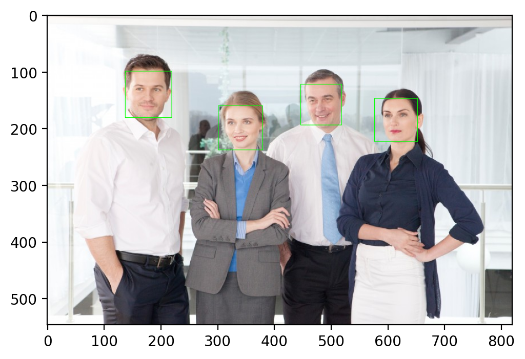
一、Haar
- # 调整参数
- img = cv2.imread('./images/001.jpg')
- cv_show('img',img)
-
- # 构造harr检测器
- face_detector = cv2.CascadeClassifier('./weights/haarcascade_frontalface_default.xml')
-
- # 转为灰度图
- img_gray = cv2.cvtColor(img,cv2.COLOR_BGR2GRAY)
- plt.imshow(img_gray,'gray')
-
- # 检测结果 上图4个人脸所以4个方框坐标
- # image
- # scaleFactor控制人脸尺寸 默认1.1
- detections = face_detector.detectMultiScale(img_gray,scaleFactor=1.3)
-
- # 解析
- for x,y,w,h in detections:
- cv2.rectangle(img,(x,y),(x+w,y+h),(0,255,0))
- plt.imshow(cv2.cvtColor(img,cv2.COLOR_BGR2RGB))

- # 调整参数
- img = cv2.imread('./images/004.jpeg')
- cv_show('img',img)
-
- # 构造harr检测器
- face_detector = cv2.CascadeClassifier('./weights/haarcascade_frontalface_default.xml')
-
- # 转为灰度图
- img_gray = cv2.cvtColor(img,cv2.COLOR_BGR2GRAY)
- plt.imshow(img_gray,'gray')
-
- # 检测结果 上图4个人脸所以4个方框坐标
- # image
- # scaleFactor控制人脸尺寸 默认1.1
- # minNeighbors 确定一个人脸框至少要有n个候选值 越高 质量越好
- # [, flags[,
- # minSize maxSize 人脸框的最大最小尺寸 如minSize=(40,40)
- detections = face_detector.detectMultiScale(img_gray,scaleFactor=1.2, minNeighbors=10)# 在质量和数量上平衡
-
- # 解析
- for x,y,w,h in detections:
- cv2.rectangle(img,(x,y),(x+w,y+h),(0,255,0))
- plt.imshow(cv2.cvtColor(img,cv2.COLOR_BGR2RGB))
上述过程中:
- scaleFactor参数:用来控制人脸框的大小,可以用它来排除一些错误检测;
- minNeighbors参数:我们给人脸框起来的时候,一般一张脸会框许多的框,假如这张脸框得越多,说明质量越好,越是一张正确的“脸”。
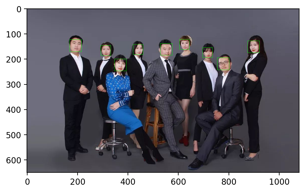
二、Hog
对于第一次使用这个功能的同学,要提前下载一下dlib。
- import dlib
-
- # 构造HOG人脸检测器 不需要参数
- hog_face_detetor = dlib.get_frontal_face_detector()
-
- # 检测人脸获取数据
- # img
- # scale类似haar的scalFactor
- detections = hog_face_detetor(img,1)
-
- # 解析获取的数据
- for face in detections:
- # 左上角
- x = face.left()
- y = face.top()
- # 右下角
- r = face.right()
- b = face.bottom()
- cv2.rectangle(img,(x,y),(r,b),(0,255,0))
- plt.imshow(cv2.cvtColor(img,cv2.COLOR_BGR2RGB))

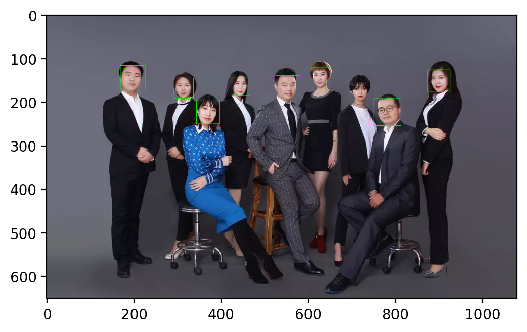
三、CNN
- import dlib
-
- # 构造CNN人脸检测器
- cnn_face_detector = dlib.cnn_face_detection_model_v1("./weights/mmod_human_face_detector.dat")
-
- # 检测人脸 参数与上一种相似
- detections = cnn_face_detector(img,1)
-
- for face in detections:
- # 左上角
- x = face.rect.left()
- y = face.rect.top()
- # 右下角
- r = face.rect.right()
- b = face.rect.bottom()
- # 置信度
- c = face.confidence
- print(c)
-
- cv2.rectangle(img,(x,y),(r,b),(0,255,0))
-
- plt.imshow(cv2.cvtColor(img,cv2.COLOR_BGR2RGB))
通过神经网络完成,这个过程中我们还可以查看每张脸检测时的置信度。
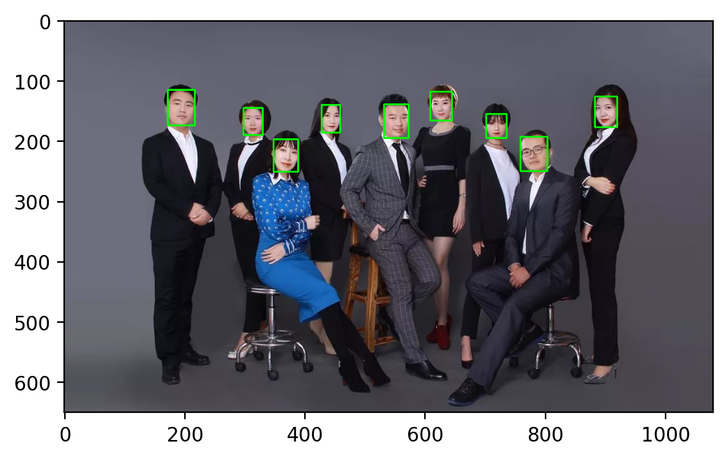
四、SSD
- # 加载模型
- face_detector = cv2.dnn.readNetFromCaffe('./weights/deploy.prototxt.txt','./weights/res10_300x300_ssd_iter_140000.caffemodel')
-
- # 原图尺寸
- img_height = img.shape[0]
- img_width = img.shape[1]
-
- # 放缩至输入尺寸
- img_resized = cv2.resize(img,(500,300))
-
- # 转为2进制
- img_blob = cv2.dnn.blobFromImage(img_resized,1.0,(500,300),(104.0,177.0,123.0))
-
- # 输入
- face_detector.setInput(img_blob)
-
- # 推理
- detections = face_detector.forward()
此时
detections.shape # (1, 1, 200, 7)说明有200个结果,后面的7则是我们做需要的一些数据,继续如下:
- # 查看人脸数量
- num_of_detections = detections.shape[2]
-
-
- img_copy = img.copy()
-
- for index in range(num_of_detections):
- # 置信度
- detections_confidence = detections[0,0,index,2]
- # 通过置信度筛选
- if detections_confidence > 0.15:
- # 位置 乘以宽高恢复大小
- locations = detections[0,0,index,3:7] * np.array([img_width,img_height,img_width,img_height])
- # 打印
- print(detections_confidence)
-
- lx,ly,rx,ry = locations.astype('int')
- # 绘制
- cv2.rectangle(img_copy,(lx,ly),(rx,ry),(0,255,0),2)
-
- plt.imshow(cv2.cvtColor(img_copy,cv2.COLOR_BGR2RGB))

五、MTCNN
- # 导入MTCNN
- from mtcnn.mtcnn import MTCNN
-
- # 记载模型
- face_detetor = MTCNN()
-
- # 检测人脸
- detections = face_detetor.detect_faces(img_cvt)
- for face in detections:
- x,y,w,h = face['box']
- cv2.rectangle(img_cvt,(x,y),(x+w,y+h),(0,255,0),2)
- plt.imshow(img_cvt)
对比
| 优势 | 劣势 | |
| Haar | 速度最快、清凉、适合算力较小的设备 | 准确度低、偶尔误报、无旋转不变性 |
| HOG+Dlib | 比Haar准确率高 | 速度比Haar低,计算量大、无旋转不变性、Dlib兼容性问题 |
| SSD | 比Haar和hog准确率高、深度学习、大小一般 | 低光照片准确率低,受肤色影响。 |
| CNN | 最准确、误报率低、轻量 | 相对于其他方法慢、计算量大、Dlib兼容性问题 |
声明:本文内容由网友自发贡献,不代表【wpsshop博客】立场,版权归原作者所有,本站不承担相应法律责任。如您发现有侵权的内容,请联系我们。转载请注明出处:https://www.wpsshop.cn/article/detail/31806
推荐阅读


相关标签

