【pytorch】从入门到构建一个分类网络超长超详细教程（附代码）_

一、pytorch入门

1、资料链接

• 内含pytorch完整的视频及资料

pytorch关于nlp的教程视频和实战：
链接：https://pan.baidu.com/s/1tbvLeUTPvxKy_gcVhiT8rw 
提取码：hgkk 

pytorch教程：
		http://pytorchchina.com/
		https://pytorch-cn.readthedocs.io/zh/latest/
		http://pytorch123.com/

b站视频链接：https://www.bilibili.com/video/av66421076
1
2
3
4
5
6
7
8
9
10

2、pytorch介绍

(1) c1_cpu和gpu速度对比.py

import time
import torch

print(torch.__version__)
print(torch.cuda.is_available)

a = torch.randn(10000, 1000)
b = torch.randn(1000, 2000)

t0 = time.time()
c = torch.matmul(a, b)
t1 = time.time()
print(a.device, t1 - t0, c.norm(2))

device = torch.device('cuda')
a = a.to(device)
b = b.to(device)

# 第一次在cuda上运行时，没有完成一些环境的初始化，因此会花费一定的时间
t0 = time.time()
c = torch.matmul(a, b)
t2 = time.time()
print(a.device, t2 - t0, c.norm(2))

# 第二次运行就是正常的gpu加速后的速度
t0 = time.time()
c = torch.matmul(a, b)
t2 = time.time()
print(a.device, t2 - t0, c.norm(2))


console:
1.2.0
<function is_available at 0x0000014EA22A72F0>
cpu 0.484722375869751 tensor(141163.7188)
cuda:0 2.04582142829895 tensor(141564.8281, device='cuda:0')
cuda:0 0.007996797561645508 tensor(141564.8281, device='cuda:0')
1
2
3
4
5
6
7
8
9
10
11
12
13
14
15
16
17
18
19
20
21
22
23
24
25
26
27
28
29
30
31
32
33
34
35
36
37

(2) c2_autograd.py — pytorch求导

import torch

x = torch.tensor(1.)
# requires_grad=True 告诉pytorch需要对a,b,c求导
a = torch.tensor(1., requires_grad=True)
b = torch.tensor(2., requires_grad=True)
c = torch.tensor(3., requires_grad=True)

y = a ** 2 * x + b * x + c

print('before: ', a.grad, b.grad, c.grad)
# 使用pytorch对y分别对a,b,c求导
grads = torch.autograd.grad(y, [a, b, c])
print('after: ', grads[0], grads[1], grads[2])


console:
before:  None None None
after:  tensor(2.) tensor(1.) tensor(1.)
1
2
3
4
5
6
7
8
9
10
11
12
13
14
15
16
17
18
19

3、张量

Tensors (张量)

Tensors 类似于 NumPy 的 ndarrays ，同时 Tensors 可以使用 GPU 进行计算。

# 其实这句函数之后，即使在低版本的python2.X，当使用print函数时，
# 须python3.X那样加括号使用。tips：python2.X中print不需要括号，
# 而在python3.X中则需要。
from __future__ import print_function
import torch
1
2
3
4
5

构造一个5×3矩阵，不初始化。

x = torch.empty(5, 3)
print(x)

console:
# 输出:
tensor(1.00000e-04 *
       [[-0.0000,  0.0000,  1.5135],
        [ 0.0000,  0.0000,  0.0000],
        [ 0.0000,  0.0000,  0.0000],
        [ 0.0000,  0.0000,  0.0000],
        [ 0.0000,  0.0000,  0.0000]])
1
2
3
4
5
6
7
8
9
10
11

构造一个随机初始化的矩阵：

x = torch.rand(5, 3)
print(x)

console:
tensor([[ 0.6291,  0.2581,  0.6414],
        [ 0.9739,  0.8243,  0.2276],
        [ 0.4184,  0.1815,  0.5131],
        [ 0.5533,  0.5440,  0.0718],
        [ 0.2908,  0.1850,  0.5297]])
1
2
3
4
5
6
7
8
9

构造一个矩阵全为 0，而且数据类型是 long.

x = torch.zeros(5, 3, dtype=torch.long)
print(x)

console:
tensor([[ 0,  0,  0],
        [ 0,  0,  0],
        [ 0,  0,  0],
        [ 0,  0,  0],
        [ 0,  0,  0]])
1
2
3
4
5
6
7
8
9

构造一个张量，直接使用数据：

x = torch.tensor([5.5, 3])
print(x)

console:
tensor([ 5.5000,  3.0000])
1
2
3
4
5

创建一个 tensor 基于已经存在的 tensor。

x = x.new_ones(5, 3, dtype=torch.double)      
# new_* methods take in sizes
print(x)

x = torch.randn_like(x, dtype=torch.float)    
# override dtype!重写数据类型
print(x)                                      
# result has the same size 最后的矩阵同样大小

console:
tensor([[ 1.,  1.,  1.],
        [ 1.,  1.,  1.],
        [ 1.,  1.,  1.],
        [ 1.,  1.,  1.],
        [ 1.,  1.,  1.]], dtype=torch.float64)
tensor([[-0.2183,  0.4477, -0.4053],
        [ 1.7353, -0.0048,  1.2177],
        [-1.1111,  1.0878,  0.9722],
        [-0.7771, -0.2174,  0.0412],
        [-2.1750,  1.3609, -0.3322]])
1
2
3
4
5
6
7
8
9
10
11
12
13
14
15
16
17
18
19
20

获取它的维度信息:

print(x.size())

console:
torch.Size([5, 3])
1
2
3
4

注意: torch.Size 是一个元组，所以它支持左右的元组操作。

加法: 方式 1

y = torch.rand(5, 3)
print(x + y)

console:
tensor([[-0.1859,  1.3970,  0.5236],
        [ 2.3854,  0.0707,  2.1970],
        [-0.3587,  1.2359,  1.8951],
        [-0.1189, -0.1376,  0.4647],
        [-1.8968,  2.0164,  0.1092]])
1
2
3
4
5
6
7
8
9

加法: 方式2

print(torch.add(x, y))

console:
tensor([[-0.1859,  1.3970,  0.5236],
        [ 2.3854,  0.0707,  2.1970],
        [-0.3587,  1.2359,  1.8951],
        [-0.1189, -0.1376,  0.4647],
        [-1.8968,  2.0164,  0.1092]])
1
2
3
4
5
6
7
8

加法: 提供一个输出 tensor 作为参数

result = torch.empty(5, 3)
# 将输出结果赋值给result
torch.add(x, y, out=result)
print(result)

console:
tensor([[-0.1859,  1.3970,  0.5236],
        [ 2.3854,  0.0707,  2.1970],
        [-0.3587,  1.2359,  1.8951],
        [-0.1189, -0.1376,  0.4647],
        [-1.8968,  2.0164,  0.1092]])
1
2
3
4
5
6
7
8
9
10
11

加法: in-place

# adds x to y
y.add_(x)
print(y)

console:
tensor([[-0.1859,  1.3970,  0.5236],
        [ 2.3854,  0.0707,  2.1970],
        [-0.3587,  1.2359,  1.8951],
        [-0.1189, -0.1376,  0.4647],
        [-1.8968,  2.0164,  0.1092]])
1
2
3
4
5
6
7
8
9
10

注意: 任何使张量会发生变化的操作都有一个前缀 ‘’。例如：x.copy(y), x.t_(), 将会改变 x.

可以使用标准的 NumPy 类似的索引操作

print(x[:, 1])

console:
tensor([ 0.4477, -0.0048,  1.0878, -0.2174,  1.3609])
1
2
3
4

改变大小：如果你想改变一个 tensor 的大小或者形状，你可以使用 torch.view:

x = torch.randn(4, 4)
y = x.view(16)
z = x.view(-1, 8)  # the size -1 is inferred from other dimensions
print(x.size(), y.size(), z.size())

console:
torch.Size([4, 4]) torch.Size([16]) torch.Size([2, 8])
1
2
3
4
5
6
7

如果你有一个元素 tensor ，使用 .item() 来获得这个 value 。

x = torch.randn(1)
print(x)
print(x.item())

console:
tensor([ 0.9422])
0.9422121644020081
1
2
3
4
5
6
7

numpy和tensor之间相互转换

• torch的tensor和numpy的array会共享他们的存储空间，修改一个会导致另一个也被修改
• cpu上除了CharTensor，都支持转换为与NumPy之间相互转换
• 将一个torch tensor 转化为numpy array

# 将torch的张量转换为numpy的数组
a = torch.ones(5)
b = a.numpy()
print(a)
print(b)

# 此处演示当修改numpy数组之后，与之相关联的tensor也会相应被修改
a.add_(1)
print(a)
print(b)

console:
tensor([1., 1., 1., 1., 1.])
[1. 1. 1. 1. 1.]
tensor([2., 2., 2., 2., 2.])
[2. 2. 2. 2. 2.]
1
2
3
4
5
6
7
8
9
10
11
12
13
14
15
16

• 将numpy数组自动更改为torch tensor

import numpy as np
import torch

a = np.ones(5)
b = torch.Tensor(a)
np.add(a, 1, out=a)
print(a)
print(b)

console:
[2. 2. 2. 2. 2.]
tensor([1., 1., 1., 1., 1.])
1
2
3
4
5
6
7
8
9
10
11
12

• tensors通过.to函数可以被移动到任何设备

if torch.cuda.is_available():
    x = torch.rand(5, 5)
    # 一个cuda设备对象
    device = torch.device("cuda")
    # 直接而在gpu上创建tensor
    y = torch.ones_like(x, device=device)
    # 或者直接用字符串.to("cuda")
    x = x.to(device)
    z = x + y
    print(z)
    print(z.to("cpu", torch.double))
    
console:
tensor([[1.4933, 1.9654, 1.8140, 1.1782, 1.9465],
        [1.4439, 1.9591, 1.0066, 1.6454, 1.2359],
        [1.2481, 1.5360, 1.9592, 1.3101, 1.6361],
        [1.0741, 1.6382, 1.2640, 1.9733, 1.7078],
        [1.8020, 1.4749, 1.4589, 1.8869, 1.2460]], device='cuda:0')
tensor([[1.4933, 1.9654, 1.8140, 1.1782, 1.9465],
        [1.4439, 1.9591, 1.0066, 1.6454, 1.2359],
        [1.2481, 1.5360, 1.9592, 1.3101, 1.6361],
        [1.0741, 1.6382, 1.2640, 1.9733, 1.7078],
        [1.8020, 1.4749, 1.4589, 1.8869, 1.2460]], dtype=torch.float64)
1
2
3
4
5
6
7
8
9
10
11
12
13
14
15
16
17
18
19
20
21
22
23

二、Autograd自动微分

1、简介

• autograd 包是 PyTorch 中所有神经网络的核心。首先让我们简要地介绍它，然后我们将会去训练我们的第一个神经网络。该 autograd 软件包为 Tensors 上的所有操作提供自动微分。它是一个由运行定义的框架，这意味着以代码运行方式定义你的后向传播，并且每次迭代都可以不同。我们从 tensor 和 gradients 来举一些例子。
• TENSOR
  • torch.Tensor 是包的核心类。如果将其属性 .requires_grad 设置为 True，则会开始跟踪针对 tensor 的所有操作。完成计算后，您可以调用 .backward() 来自动计算所有梯度。该张量的梯度将累积到 .grad 属性中。
  • 要停止 tensor 历史记录的跟踪，您可以调用 .detach()，它将其与计算历史记录分离，并防止将来的计算被跟踪。
  • 要停止跟踪历史记录（和使用内存），您还可以将代码块使用 with torch.no_grad(): 包装起来。在评估模型时，这是特别有用，因为模型在训练阶段具有 requires_grad = True 的可训练参数有利于调参，但在评估阶段我们不需要梯度。
  • 还有一个类对于 autograd 实现非常重要那就是 Function。Tensor 和 Function 互相连接并构建一个非循环图，它保存整个完整的计算过程的历史信息。每个张量都有一个 .grad_fn 属性保存着创建了张量的 Function 的引用，（如果用户自己创建张量，则grad_fn 是 None ）。
  • 如果你想计算导数，你可以调用 Tensor.backward()。如果 Tensor 是标量（即它包含一个元素数据），则不需要指定任何参数backward()，但是如果它有更多元素，则需要指定一个gradient 参数来指定张量的形状。

2、怎么用？

• 跟踪Tensor上的所有操作：设置属性requires_grad=True
• 自动计算所有梯度：调用.backward()
• 停止跟踪Tensor：
  • 方式一：调用detach()
  • 方式二：代码块：with torch.no grad

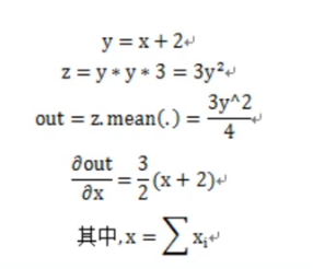
创建一个张量，设置 requires_grad=True 来跟踪与它相关的计算

x = torch.ones(2, 2, requires_grad=True)
print(x)
# 针对张量做一个操作
y = x + 2
print(y)
# y 作为操作的结果被创建，所以它有 grad_fn
print(y.grad_fn)
# 针对张量做更多操作
z = y * y * 3
out = z.mean()
print(z, out)

console:
tensor([[1., 1.],
        [1., 1.]], requires_grad=True)
# 每个张量都有一个 .grad_fn 属性保存着创建了张量的 Function 的引用
tensor([[3., 3.],
        [3., 3.]], grad_fn=<AddBackward0>) <AddBackward0 object at 0x000001989F20D7B8>
tensor([[27., 27.],
        [27., 27.]], grad_fn=<MulBackward0>) tensor(27., grad_fn=<MeanBackward0>)
1
2
3
4
5
6
7
8
9
10
11
12
13
14
15
16
17
18
19
20

.requires_grad_( … ) 会改变张量的 requires_grad 标记。

• 如果没有提供相应的参数,输入的标记默认为 False。

import torch

a = torch.randn(2, 2)
a = ((a * .3) / (a - 1))
print(a.requires_grad)
a.requires_grad_(True)
print(a.requires_grad)
b = (a * a).sum()
print(b.grad_fn)

console:
False
True
<SumBackward0 object at 0x000001B498D8D7B8>
1
2
3
4
5
6
7
8
9
10
11
12
13
14

梯度：

• backward函数是反向传播的入口点，在需要被求导的节点上调用backward函数会计算梯度值到相应的节点上。backward需要一个重要的参数grad_tensor，但如果节点只含有一个标量值，这个参数就可以忽略。我们现在后向传播，因为输出包含了一个标量，所以out.backward() 等同于 out.backward(torch.tensor(1.))， 否者就会报如下错误：

backward should be called only on a scalar (i.e, 1-element tensor) or with gradient w.r.t the variable
1

import torch
x = torch.ones(2, 2, requires_grad=True)
print(x)
# 针对张量做一个操作
y = x + 2
print(y)
# y 作为操作的结果被创建，所以它有 grad_fn
print(y.grad_fn)
# 针对张量做更多操作
z = y * y * 3
out = z.mean()
print(z)
print(out)

out.backward()
print(x.grad)

console:

tensor([[1., 1.],
        [1., 1.]], requires_grad=True)
tensor([[3., 3.],
        [3., 3.]], grad_fn=<AddBackward0>)
<AddBackward0 object at 0x00000210E6595080>
tensor([[27., 27.],
        [27., 27.]], grad_fn=<MulBackward0>)
tensor(27., grad_fn=<MeanBackward0>)
tensor([[4.5000, 4.5000],
        [4.5000, 4.5000]])
1
2
3
4
5
6
7
8
9
10
11
12
13
14
15
16
17
18
19
20
21
22
23
24
25
26
27
28
29

• 原理解释：
  
  
• 英文版解释
  
• 中文版解释：
  
  

雅可比向量的例子：

import torch
# .requires_grad=True 的张量自动求导。
x = torch.randn(3, requires_grad=True)
y = x * 2
while y.data.norm() < 1000:
    y = y * 2
print(x)
print(y)
# 现在在这种情况下，y 不再是一个标量。torch.autograd 不能够直接计算整个雅可比，
# 但是如果我们只想要雅可比向量积，只需要简单的传递向量给 backward 作为参数。
v = torch.tensor([0.1, 1.0, 0.0001], dtype=torch.float)
y.backward(v)
print(x.grad)
# 你可以通过将代码包裹在 with torch.no_grad()，来停止对从跟踪历史中的
# .requires_grad=True 的张量自动求导。
print(x.requires_grad)
print((x ** 2).requires_grad)
with torch.no_grad():
    print((x ** 2).requires_grad)

console:

tensor([ 0.2052,  0.6057, -0.6355], requires_grad=True)
tensor([  420.3014,  1240.4666, -1301.4670], grad_fn=<MulBackward0>)
tensor([2.0480e+02, 2.0480e+03, 2.0480e-01])
True
True
False
1
2
3
4
5
6
7
8
9
10
11
12
13
14
15
16
17
18
19
20
21
22
23
24
25
26
27
28

三、PyTorch神经网络

1、简介

• 神经网络可以通过 torch.nn 包来构建。

• 现在对于自动梯度(autograd)有一些了解，神经网络是基于自动梯度 (autograd)来定义一些模型。一个 nn.Module 包括层和一个方法 forward(input) 它会返回输出(output)。

• 例如，看一下数字图片识别的网络：
  

• 这是一个简单的前馈神经网络，它接收输入，让输入一个接着一个的通过一些层，最后给出输出。

• 一个典型的神经网络训练过程包括以下几点：

  • 1.定义一个包含可训练参数的神经网络
  • 2.迭代整个输入
  • 3.通过神经网络处理输入
  • 4.计算损失(loss)
  • 5.反向传播梯度到神经网络的参数
  • 6.更新网络的参数，典型的用一个简单的更新方法：weight = weight - learning_rate *gradient

2、神经网络各参数意义

3、定义神经网络

# -*- coding: utf-8 -*-
"""
Neural Networks
===============

Neural networks can be constructed using the ``torch.nn`` package.

Now that you had a glimpse of ``autograd``, ``nn`` depends on
``autograd`` to define models and differentiate them.
An ``nn.Module`` contains layers, and a method ``forward(input)`` that
returns the ``output``.

For example, look at this network that classifies digit images:

.. figure:: /_static/img/mnist.png
   :alt: convnet

   convnet

It is a simple feed-forward network. It takes the input, feeds it
through several layers one after the other, and then finally gives the
output.

A typical training procedure for a neural network is as follows:

- Define the neural network that has some learnable parameters (or
  weights)
- Iterate over a dataset of inputs
- Process input through the network
- Compute the loss (how far is the output from being correct)
- Propagate gradients back into the network’s parameters
- Update the weights of the network, typically using a simple update rule:
  ``weight = weight - learning_rate * gradient``

Define the network
------------------

Let’s define this network:
"""
import torch
import torch.nn as nn
import torch.nn.functional as F


class Net(nn.Module):

    def __init__(self):
        super(Net, self).__init__()
        # 1 input image channel, 6 output channels, 5x5 square convolution
        # kernel
        self.conv1 = nn.Conv2d(1, 6, 5)
        self.conv2 = nn.Conv2d(6, 16, 5)
        # an affine operation: y = Wx + b
        self.fc1 = nn.Linear(16 * 5 * 5, 120)
        self.fc2 = nn.Linear(120, 84)
        self.fc3 = nn.Linear(84, 10)

    def forward(self, x):
        # Max pooling over a (2, 2) window
        x = F.max_pool2d(F.relu(self.conv1(x)), (2, 2))
        # If the size is a square you can only specify a single number
        x = F.max_pool2d(F.relu(self.conv2(x)), 2)
        x = x.view(-1, self.num_flat_features(x))
        x = F.relu(self.fc1(x))
        x = F.relu(self.fc2(x))
        x = self.fc3(x)
        return x

    def num_flat_features(self, x):
        size = x.size()[1:]  # all dimensions except the batch dimension
        num_features = 1
        for s in size:
            num_features *= s
        return num_features


net = Net()
print(net)
print('---------------------')

########################################################################
# You just have to define the ``forward`` function, and the ``backward``
# function (where gradients are computed) is automatically defined for you
# using ``autograd``.
# You can use any of the Tensor operations in the ``forward`` function.
#
# The learnable parameters of a model are returned by ``net.parameters()``

# 一个模型可训练的参数可以通过调用 net.parameters() 返回：
params = list(net.parameters())
print(len(params))
print(params[0].size())  # conv1's .weight
print('---------------------')


########################################################################
# Let try a random 32x32 input
# Note: Expected input size to this net(LeNet) is 32x32. To use this net on
# MNIST dataset, please resize the images from the dataset to 32x32.

# 让我们尝试随机生成一个 32x32 的输入。注意：期望的输入维度是 32x32 。
# 为了使用这个网络在 MNIST 数据及上，你需要把数据集中的图片维度修改为 32x32。
input = torch.randn(1, 1, 32, 32)
out = net(input)
print(out)
print('---------------------')


########################################################################
# Zero the gradient buffers of all parameters and backprops with random
# gradients:

# 把所有参数梯度缓存器置零，用随机的梯度来反向传播
net.zero_grad()
out.backward(torch.randn(1, 10))
print('---------------------')


########################################################################
# .. note::
#
#     ``torch.nn`` only supports mini-batches. The entire ``torch.nn``
#     package only supports inputs that are a mini-batch of samples, and not
#     a single sample.
#
#     For example, ``nn.Conv2d`` will take in a 4D Tensor of
#     ``nSamples x nChannels x Height x Width``.
#
#     If you have a single sample, just use ``input.unsqueeze(0)`` to add
#     a fake batch dimension.
#
# Before proceeding further, let's recap all the classes you’ve seen so far.
#
# **Recap:**
#   -  ``torch.Tensor`` - A *multi-dimensional array* with support for autograd
#      operations like ``backward()``. Also *holds the gradient* w.r.t. the
#      tensor.
#   -  ``nn.Module`` - Neural network module. *Convenient way of
#      encapsulating parameters*, with helpers for moving them to GPU,
#      exporting, loading, etc.
#   -  ``nn.Parameter`` - A kind of Tensor, that is *automatically
#      registered as a parameter when assigned as an attribute to a*
#      ``Module``.
#   -  ``autograd.Function`` - Implements *forward and backward definitions
#      of an autograd operation*. Every ``Tensor`` operation, creates at
#      least a single ``Function`` node, that connects to functions that
#      created a ``Tensor`` and *encodes its history*.
#
# **At this point, we covered:**
#   -  Defining a neural network
#   -  Processing inputs and calling backward
#
# **Still Left:**
#   -  Computing the loss
#   -  Updating the weights of the network
#
# Loss Function
# -------------
# A loss function takes the (output, target) pair of inputs, and computes a
# value that estimates how far away the output is from the target.
#
# There are several different
# `loss functions <https://pytorch.org/docs/nn.html#loss-functions>`_ under the
# nn package .
# A simple loss is: ``nn.MSELoss`` which computes the mean-squared error
# between the input and the target.
#
# For example:

output = net(input)
target = torch.randn(10)  # a dummy target, for example
target = target.view(1, -1)  # make it the same shape as output
criterion = nn.MSELoss()

loss = criterion(output, target)
print(loss)
print('---------------------')


########################################################################
# Now, if you follow ``loss`` in the backward direction, using its
# ``.grad_fn`` attribute, you will see a graph of computations that looks
# like this:
#
# ::
#
#     input -> conv2d -> relu -> maxpool2d -> conv2d -> relu -> maxpool2d
#           -> view -> linear -> relu -> linear -> relu -> linear
#           -> MSELoss
#           -> loss
#
# So, when we call ``loss.backward()``, the whole graph is differentiated
# w.r.t. the loss, and all Tensors in the graph that has ``requires_grad=True``
# will have their ``.grad`` Tensor accumulated with the gradient.
#
# For illustration, let us follow a few steps backward:

print(loss.grad_fn)  # MSELoss
print(loss.grad_fn.next_functions[0][0])  # Linear
print(loss.grad_fn.next_functions[0][0].next_functions[0][0])  # ReLU
print('---------------------')


########################################################################
# Backprop
# --------
# To backpropagate the error all we have to do is to ``loss.backward()``.
# You need to clear the existing gradients though, else gradients will be
# accumulated to existing gradients.
#
#
# Now we shall call ``loss.backward()``, and have a look at conv1's bias
# gradients before and after the backward.


net.zero_grad()     # zeroes the gradient buffers of all parameters

print('conv1.bias.grad before backward')
print(net.conv1.bias.grad)

loss.backward()

print('conv1.bias.grad after backward')
print(net.conv1.bias.grad)
print('---------------------')


########################################################################
# Now, we have seen how to use loss functions.
#
# **Read Later:**
#
#   The neural network package contains various modules and loss functions
#   that form the building blocks of deep neural networks. A full list with
#   documentation is `here <https://pytorch.org/docs/nn>`_.
#
# **The only thing left to learn is:**
#
#   - Updating the weights of the network
#
# Update the weights
# ------------------
# The simplest update rule used in practice is the Stochastic Gradient
# Descent (SGD):
#
#      ``weight = weight - learning_rate * gradient``
#
# We can implement this using simple python code:
#
# .. code:: python
#
#     learning_rate = 0.01
#     for f in net.parameters():
#         f.data.sub_(f.grad.data * learning_rate)
#
# However, as you use neural networks, you want to use various different
# update rules such as SGD, Nesterov-SGD, Adam, RMSProp, etc.
# To enable this, we built a small package: ``torch.optim`` that
# implements all these methods. Using it is very simple:

import torch.optim as optim

# create your optimizer
optimizer = optim.SGD(net.parameters(), lr=0.01)

# in your training loop:
optimizer.zero_grad()   # zero the gradient buffers
output = net(input)
loss = criterion(output, target)
loss.backward()
optimizer.step()    # Does the update
print('---------------------')


###############################################################
# .. Note::
#
#       Observe how gradient buffers had to be manually set to zero using
#       ``optimizer.zero_grad()``. This is because gradients are accumulated
#       as explained in `Backprop`_ section.


console:

Net(
  (conv1): Conv2d(1, 6, kernel_size=(5, 5), stride=(1, 1))
  (conv2): Conv2d(6, 16, kernel_size=(5, 5), stride=(1, 1))
  (fc1): Linear(in_features=400, out_features=120, bias=True)
  (fc2): Linear(in_features=120, out_features=84, bias=True)
  (fc3): Linear(in_features=84, out_features=10, bias=True)
)
---------------------
10
torch.Size([6, 1, 5, 5])
---------------------
tensor([[-0.0588, -0.0427, -0.1616,  0.0437,  0.0163,  0.0543, -0.1478, -0.0592,
         -0.0509,  0.0549]], grad_fn=<AddmmBackward>)
---------------------
---------------------
tensor(0.4980, grad_fn=<MseLossBackward>)
---------------------
<MseLossBackward object at 0x0000024FE0C6A8D0>
<AddmmBackward object at 0x0000024F8313D4A8>
<AccumulateGrad object at 0x0000024FE0C6A8D0>
---------------------
conv1.bias.grad before backward
tensor([0., 0., 0., 0., 0., 0.])
conv1.bias.grad after backward
tensor([-5.8280e-03,  1.1338e-02,  1.7925e-03, -6.9680e-07,  9.8157e-03,
         2.1737e-03])
---------------------
---------------------
1
2
3
4
5
6
7
8
9
10
11
12
13
14
15
16
17
18
19
20
21
22
23
24
25
26
27
28
29
30
31
32
33
34
35
36
37
38
39
40
41
42
43
44
45
46
47
48
49
50
51
52
53
54
55
56
57
58
59
60
61
62
63
64
65
66
67
68
69
70
71
72
73
74
75
76
77
78
79
80
81
82
83
84
85
86
87
88
89
90
91
92
93
94
95
96
97
98
99
100
101
102
103
104
105
106
107
108
109
110
111
112
113
114
115
116
117
118
119
120
121
122
123
124
125
126
127
128
129
130
131
132
133
134
135
136
137
138
139
140
141
142
143
144
145
146
147
148
149
150
151
152
153
154
155
156
157
158
159
160
161
162
163
164
165
166
167
168
169
170
171
172
173
174
175
176
177
178
179
180
181
182
183
184
185
186
187
188
189
190
191
192
193
194
195
196
197
198
199
200
201
202
203
204
205
206
207
208
209
210
211
212
213
214
215
216
217
218
219
220
221
222
223
224
225
226
227
228
229
230
231
232
233
234
235
236
237
238
239
240
241
242
243
244
245
246
247
248
249
250
251
252
253
254
255
256
257
258
259
260
261
262
263
264
265
266
267
268
269
270
271
272
273
274
275
276
277
278
279
280
281
282
283
284
285
286
287
288
289
290
291
292
293
294
295
296
297
298
299
300
301
302
303
304
305
306
307
308
309
310
311
312

你刚定义了一个前馈函数，然后反向传播函数被自动通过 autograd 定义了。你可以使用任何张量操作在前馈函数上。

4、损失函数

• 一个损失函数需要一对输入：模型输出和目标，然后计算一个值来评估输出距离目标有多远。
• 有一些不同的损失函数在 nn 包中。一个简单的损失函数就是 nn.MSELoss ，这计算了输入与目标的均方误差。

output = net(input)
target = torch.randn(10)  # a dummy target, for example
target = target.view(1, -1)  # make it the same shape as output
criterion = nn.MSELoss()

loss = criterion(output, target)
print(loss)

console:

tensor(0.6660, grad_fn=<MseLossBackward>)
1
2
3
4
5
6
7
8
9
10
11

• 现在，如果你跟随损失到反向传播路径，可以使用它的 .grad_fn 属性，你将会看到一个这样的计算图：

input -> conv2d -> relu -> maxpool2d -> conv2d -> relu -> maxpool2d
      -> view -> linear -> relu -> linear -> relu -> linear
      -> MSELoss
      -> loss
1
2
3
4

• 所以，当我们调用 loss.backward()，整个图都会微分，而且所有的在图中的requires_grad=True 的张量将会让他们的 grad 张量累计梯度。
• 为了演示，我们将跟随以下步骤来反向传播。

print(loss.grad_fn)  # MSELoss
print(loss.grad_fn.next_functions[0][0])  # Linear
print(loss.grad_fn.next_functions[0][0].next_functions[0][0])  # ReLU

console:
<MseLossBackward object at 0x0000019183144C18>
<AddmmBackward object at 0x0000019183144D30>
<AccumulateGrad object at 0x0000019183144D30>
1
2
3
4
5
6
7
8

5、反向传播

• 为了实现反向传播损失，我们所有需要做的事情仅仅是使用 loss.backward()。你需要清空现存的梯度，要不然帝都将会和现存的梯度累计到一起。
• 现在我们调用 loss.backward() ，然后看一下 con1 的偏置项在反向传播之前和之后的变化。

net.zero_grad()     # zeroes the gradient buffers of all parameters

print('conv1.bias.grad before backward')
print(net.conv1.bias.grad)

loss.backward()

print('conv1.bias.grad after backward')
print(net.conv1.bias.grad)

console:

conv1.bias.grad before backward
tensor([0., 0., 0., 0., 0., 0.])
conv1.bias.grad after backward
tensor([-5.8280e-03,  1.1338e-02,  1.7925e-03, -6.9680e-07,  9.8157e-03,
         2.1737e-03])
1
2
3
4
5
6
7
8
9
10
11
12
13
14
15
16
17

• 现在我们看到了，如何使用损失函数。唯一剩下的事情就是更新神经网络的参数。更新神经网络参数：最简单的更新规则就是随机梯度下降。

weight = weight - learning_rate * gradient
1

• 我们可以使用 python 来实现这个规则：

learning_rate = 0.01
for f in net.parameters():
    f.data.sub_(f.grad.data * learning_rate)
1
2
3

• 尽管如此，如果你是用神经网络，你想使用不同的更新规则，类似于 SGD, Nesterov-SGD, Adam, RMSProp, 等。为了让这可行，我们建立了一个小包：torch.optim 实现了所有的方法。使用它非常的简单。

import torch.optim as optim

# create your optimizer
optimizer = optim.SGD(net.parameters(), lr=0.01)

# in your training loop:
optimizer.zero_grad()   # zero the gradient buffers
output = net(input)
loss = criterion(output, target)
loss.backward()
optimizer.step()    # Does the update
1
2
3
4
5
6
7
8
9
10
11

四、CIFAR10图像分类

1、简介

• 通常来说，当你处理图像，文本，语音或者视频数据时，你可以使用标准 python 包将数据加载成 numpy 数组格式，然后将这个数组转换成 torch.*Tensor

  • 对于图像，可以用 Pillow，OpenCV
  • 对于语音，可以用 scipy，librosa
  • 对于文本，可以直接用 Python 或 Cython 基础数据加载模块，或者用 NLTK 和 SpaCy

• 特别是对于视觉，我们已经创建了一个叫做 totchvision 的包，该包含有支持加载类似Imagenet，CIFAR10，MNIST 等公共数据集的数据加载模块 torchvision.datasets 和支持加载图像数据数据转换模块 torch.utils.data.DataLoader。

• 这提供了极大的便利，并且避免了编写“样板代码”。

• 对于本教程，我们将使用CIFAR10数据集，它包含十个类别：‘airplane’, ‘automobile’, ‘bird’, ‘cat’, ‘deer’, ‘dog’, ‘frog’, ‘horse’, ‘ship’, ‘truck’。CIFAR-10 中的图像尺寸为33232，也就是RGB的3层颜色通道，每层通道内的尺寸为32*32。
  

2、函数介绍

• make_grid的作用是将若干幅图像拼成一幅图像。其中padding的作用就是子图像与子图像之间的pad有多宽。

3、训练一个图像分类器

• 我们将按次序的做如下几步：
  • 使用torchvision加载并且归一化CIFAR10的训练和测试数据集
  • 定义一个卷积神经网络
  • 定义一个损失函数
  • 在训练样本数据上训练网络
  • 在测试样本数据上测试网络

整体神经网络

# -*- coding: utf-8 -*-
"""
Training a Classifier
=====================

This is it. You have seen how to define neural networks, compute loss and make
updates to the weights of the network.

Now you might be thinking,

What about data?
----------------

Generally, when you have to deal with image, text, audio or video data,
you can use standard python packages that load data into a numpy array.
Then you can convert this array into a ``torch.*Tensor``.

-  For images, packages such as Pillow, OpenCV are useful
-  For audio, packages such as scipy and librosa
-  For text, either raw Python or Cython based loading, or NLTK and
   SpaCy are useful

Specifically for vision, we have created a package called
``torchvision``, that has data loaders for common datasets such as
Imagenet, CIFAR10, MNIST, etc. and data transformers for images, viz.,
``torchvision.datasets`` and ``torch.utils.data.DataLoader``.

This provides a huge convenience and avoids writing boilerplate code.

For this tutorial, we will use the CIFAR10 dataset.
It has the classes: ‘airplane’, ‘automobile’, ‘bird’, ‘cat’, ‘deer’,
‘dog’, ‘frog’, ‘horse’, ‘ship’, ‘truck’. The images in CIFAR-10 are of
size 3x32x32, i.e. 3-channel color images of 32x32 pixels in size.

.. figure:: /_static/img/cifar10.png
   :alt: cifar10

   cifar10


Training an image classifier
----------------------------

We will do the following steps in order:

1. Load and normalizing the CIFAR10 training and test datasets using
   ``torchvision``
2. Define a Convolutional Neural Network
3. Define a loss function
4. Train the network on the training data
5. Test the network on the test data

1. Loading and normalizing CIFAR10
^^^^^^^^^^^^^^^^^^^^^^^^^^^^^^^^^^

Using ``torchvision``, it’s extremely easy to load CIFAR10.
"""
import torch
import torchvision
import torchvision.transforms as transforms

########################################################################
# The output of torchvision datasets are PILImage images of range [0, 1].
# We transform them to Tensors of normalized range [-1, 1].

transform = transforms.Compose(
    [transforms.ToTensor(),
     transforms.Normalize((0.5, 0.5, 0.5), (0.5, 0.5, 0.5))])

trainset = torchvision.datasets.CIFAR10(root='./data', train=True,
                                        download=True, transform=transform)
trainloader = torch.utils.data.DataLoader(trainset, batch_size=4,
                                          shuffle=True, num_workers=2)

testset = torchvision.datasets.CIFAR10(root='./data', train=False,
                                       download=True, transform=transform)
testloader = torch.utils.data.DataLoader(testset, batch_size=4,
                                         shuffle=False, num_workers=2)

classes = ('plane', 'car', 'bird', 'cat',
           'deer', 'dog', 'frog', 'horse', 'ship', 'truck')

########################################################################
# Let us show some of the training images, for fun.

import matplotlib.pyplot as plt
import numpy as np

# functions to show an image


def imshow(img):
    img = img / 2 + 0.5     # unnormalize
    npimg = img.numpy()
    plt.imshow(np.transpose(npimg, (1, 2, 0)))
    plt.show()


# get some random training images
dataiter = iter(trainloader)
images, labels = dataiter.next()

# show images
imshow(torchvision.utils.make_grid(images))
# print labels
print(' '.join('%5s' % classes[labels[j]] for j in range(4)))


########################################################################
# 2. Define a Convolutional Neural Network
# ^^^^^^^^^^^^^^^^^^^^^^^^^^^^^^^^^^^^^^
# Copy the neural network from the Neural Networks section before and modify it to
# take 3-channel images (instead of 1-channel images as it was defined).

import torch.nn as nn
import torch.nn.functional as F


class Net(nn.Module):
    def __init__(self):
        super(Net, self).__init__()
        self.conv1 = nn.Conv2d(3, 6, 5)
        self.pool = nn.MaxPool2d(2, 2)
        self.conv2 = nn.Conv2d(6, 16, 5)
        self.fc1 = nn.Linear(16 * 5 * 5, 120)
        self.fc2 = nn.Linear(120, 84)
        self.fc3 = nn.Linear(84, 10)

    def forward(self, x):
        x = self.pool(F.relu(self.conv1(x)))
        x = self.pool(F.relu(self.conv2(x)))
        x = x.view(-1, 16 * 5 * 5)
        x = F.relu(self.fc1(x))
        x = F.relu(self.fc2(x))
        x = self.fc3(x)
        return x


net = Net()

########################################################################
# 3. Define a Loss function and optimizer
# ^^^^^^^^^^^^^^^^^^^^^^^^^^^^^^^^^^^^^^^
# Let's use a Classification Cross-Entropy loss and SGD with momentum.

import torch.optim as optim

criterion = nn.CrossEntropyLoss()
optimizer = optim.SGD(net.parameters(), lr=0.001, momentum=0.9)

########################################################################
# 4. Train the network
# ^^^^^^^^^^^^^^^^^^^^
#
# This is when things start to get interesting.
# We simply have to loop over our data iterator, and feed the inputs to the
# network and optimize.

for epoch in range(2):  # loop over the dataset multiple times

    running_loss = 0.0
    for i, data in enumerate(trainloader, 0):
        # get the inputs
        inputs, labels = data

        # zero the parameter gradients
        optimizer.zero_grad()

        # forward + backward + optimize
        outputs = net(inputs)
        loss = criterion(outputs, labels)
        loss.backward()
        optimizer.step()

        # print statistics
        running_loss += loss.item()
        if i % 2000 == 1999:    # print every 2000 mini-batches
            print('[%d, %5d] loss: %.3f' %
                  (epoch + 1, i + 1, running_loss / 2000))
            running_loss = 0.0

print('Finished Training')

########################################################################
# 5. Test the network on the test data
# ^^^^^^^^^^^^^^^^^^^^^^^^^^^^^^^^^^^^
#
# We have trained the network for 2 passes over the training dataset.
# But we need to check if the network has learnt anything at all.
#
# We will check this by predicting the class label that the neural network
# outputs, and checking it against the ground-truth. If the prediction is
# correct, we add the sample to the list of correct predictions.
#
# Okay, first step. Let us display an image from the test set to get familiar.

dataiter = iter(testloader)
images, labels = dataiter.next()

# print images
imshow(torchvision.utils.make_grid(images))
print('GroundTruth: ', ' '.join('%5s' % classes[labels[j]] for j in range(4)))

########################################################################
# Okay, now let us see what the neural network thinks these examples above are:

outputs = net(images)

########################################################################
# The outputs are energies for the 10 classes.
# Higher the energy for a class, the more the network
# thinks that the image is of the particular class.
# So, let's get the index of the highest energy:
_, predicted = torch.max(outputs, 1)

print('Predicted: ', ' '.join('%5s' % classes[predicted[j]]
                              for j in range(4)))

########################################################################
# The results seem pretty good.
#
# Let us look at how the network performs on the whole dataset.

correct = 0
total = 0
with torch.no_grad():
    for data in testloader:
        images, labels = data
        outputs = net(images)
        _, predicted = torch.max(outputs.data, 1)
        total += labels.size(0)
        correct += (predicted == labels).sum().item()

print('Accuracy of the network on the 10000 test images: %d %%' % (
    100 * correct / total))

########################################################################
# That looks waaay better than chance, which is 10% accuracy (randomly picking
# a class out of 10 classes).
# Seems like the network learnt something.
#
# Hmmm, what are the classes that performed well, and the classes that did
# not perform well:

class_correct = list(0. for i in range(10))
class_total = list(0. for i in range(10))
with torch.no_grad():
    for data in testloader:
        images, labels = data
        outputs = net(images)
        _, predicted = torch.max(outputs, 1)
        c = (predicted == labels).squeeze()
        for i in range(4):
            label = labels[i]
            class_correct[label] += c[i].item()
            class_total[label] += 1


for i in range(10):
    print('Accuracy of %5s : %2d %%' % (
        classes[i], 100 * class_correct[i] / class_total[i]))

########################################################################
# Okay, so what next?
#
# How do we run these neural networks on the GPU?
#
# Training on GPU
# ----------------
# Just like how you transfer a Tensor on to the GPU, you transfer the neural
# net onto the GPU.
#
# Let's first define our device as the first visible cuda device if we have
# CUDA available:

device = torch.device("cuda:0" if torch.cuda.is_available() else "cpu")

# Assume that we are on a CUDA machine, then this should print a CUDA device:

print(device)

########################################################################
# The rest of this section assumes that `device` is a CUDA device.
#
# Then these methods will recursively go over all modules and convert their
# parameters and buffers to CUDA tensors:
#
# .. code:: python
#
#     net.to(device)
#
#
# Remember that you will have to send the inputs and targets at every step
# to the GPU too:
#
# .. code:: python
#
#         inputs, labels = inputs.to(device), labels.to(device)
#
# Why dont I notice MASSIVE speedup compared to CPU? Because your network
# is realllly small.
#
# **Exercise:** Try increasing the width of your network (argument 2 of
# the first ``nn.Conv2d``, and argument 1 of the second ``nn.Conv2d`` –
# they need to be the same number), see what kind of speedup you get.
#
# **Goals achieved**:
#
# - Understanding PyTorch's Tensor library and neural networks at a high level.
# - Train a small neural network to classify images
#
# Training on multiple GPUs
# -------------------------
# If you want to see even more MASSIVE speedup using all of your GPUs,
# please check out :doc:`data_parallel_tutorial`.
#
# Where do I go next?
# -------------------
#
# -  :doc:`Train neural nets to play video games </intermediate/reinforcement_q_learning>`
# -  `Train a state-of-the-art ResNet network on imagenet`_
# -  `Train a face generator using Generative Adversarial Networks`_
# -  `Train a word-level language model using Recurrent LSTM networks`_
# -  `More examples`_
# -  `More tutorials`_
# -  `Discuss PyTorch on the Forums`_
# -  `Chat with other users on Slack`_
#
# .. _Train a state-of-the-art ResNet network on imagenet: https://github.com/pytorch/examples/tree/master/imagenet
# .. _Train a face generator using Generative Adversarial Networks: https://github.com/pytorch/examples/tree/master/dcgan
# .. _Train a word-level language model using Recurrent LSTM networks: https://github.com/pytorch/examples/tree/master/word_language_model
# .. _More examples: https://github.com/pytorch/examples
# .. _More tutorials: https://github.com/pytorch/tutorials
# .. _Discuss PyTorch on the Forums: https://discuss.pytorch.org/
# .. _Chat with other users on Slack: https://pytorch.slack.com/messages/beginner/

console:
Files already downloaded and verified
Files already downloaded and verified
plane   cat  deer horse
[1,  2000] loss: 2.286
[1,  4000] loss: 1.921
[1,  6000] loss: 1.731
[1,  8000] loss: 1.616
[1, 10000] loss: 1.568
[1, 12000] loss: 1.484
[2,  2000] loss: 1.408
[2,  4000] loss: 1.382
[2,  6000] loss: 1.345
[2,  8000] loss: 1.322
[2, 10000] loss: 1.304
[2, 12000] loss: 1.271
Finished Training
GroundTruth:    cat  ship  ship plane
Predicted:    cat  ship plane plane
Accuracy of the network on the 10000 test images: 55 %
Accuracy of plane : 63 %
Accuracy of   car : 50 %
Accuracy of  bird : 38 %
Accuracy of   cat : 41 %
Accuracy of  deer : 37 %
Accuracy of   dog : 41 %
Accuracy of  frog : 77 %
Accuracy of horse : 63 %
Accuracy of  ship : 70 %
Accuracy of truck : 71 %
cuda:0
1
2
3
4
5
6
7
8
9
10
11
12
13
14
15
16
17
18
19
20
21
22
23
24
25
26
27
28
29
30
31
32
33
34
35
36
37
38
39
40
41
42
43
44
45
46
47
48
49
50
51
52
53
54
55
56
57
58
59
60
61
62
63
64
65
66
67
68
69
70
71
72
73
74
75
76
77
78
79
80
81
82
83
84
85
86
87
88
89
90
91
92
93
94
95
96
97
98
99
100
101
102
103
104
105
106
107
108
109
110
111
112
113
114
115
116
117
118
119
120
121
122
123
124
125
126
127
128
129
130
131
132
133
134
135
136
137
138
139
140
141
142
143
144
145
146
147
148
149
150
151
152
153
154
155
156
157
158
159
160
161
162
163
164
165
166
167
168
169
170
171
172
173
174
175
176
177
178
179
180
181
182
183
184
185
186
187
188
189
190
191
192
193
194
195
196
197
198
199
200
201
202
203
204
205
206
207
208
209
210
211
212
213
214
215
216
217
218
219
220
221
222
223
224
225
226
227
228
229
230
231
232
233
234
235
236
237
238
239
240
241
242
243
244
245
246
247
248
249
250
251
252
253
254
255
256
257
258
259
260
261
262
263
264
265
266
267
268
269
270
271
272
273
274
275
276
277
278
279
280
281
282
283
284
285
286
287
288
289
290
291
292
293
294
295
296
297
298
299
300
301
302
303
304
305
306
307
308
309
310
311
312
313
314
315
316
317
318
319
320
321
322
323
324
325
326
327
328
329
330
331
332
333
334
335
336
337
338
339
340
341
342
343
344
345
346
347
348
349
350
351
352
353
354
355
356
357
358
359
360
361
362
363
364
365
366
367

下载数据集

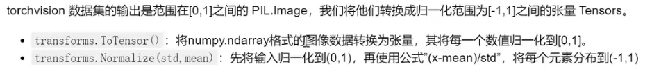
• 加载并归一化 CIFAR10 使用 torchvision ,用它来加载 CIFAR10 数据非常简单。

import torch
import torchvision
import torchvision.transforms as transforms

transform = transforms.Compose(
    [transforms.ToTensor(),
     transforms.Normalize((0.5, 0.5, 0.5), (0.5, 0.5, 0.5))])

trainset = torchvision.datasets.CIFAR10(root='./data', train=True,
                                        download=True, transform=transform)
trainloader = torch.utils.data.DataLoader(trainset, batch_size=4,
                                          shuffle=True, num_workers=2)

testset = torchvision.datasets.CIFAR10(root='./data', train=False,
                                       download=True, transform=transform)
testloader = torch.utils.data.DataLoader(testset, batch_size=4,
                                         shuffle=False, num_workers=2)

classes = ('plane', 'car', 'bird', 'cat',
           'deer', 'dog', 'frog', 'horse', 'ship', 'truck')
1
2
3
4
5
6
7
8
9
10
11
12
13
14
15
16
17
18
19
20

展示其中的一些训练图片

import matplotlib.pyplot as plt
import numpy as np

# functions to show an image


def imshow(img):
    print(img)
    img = img / 2 + 0.5     # unnormalize
    npimg = img.numpy()
    print(npimg)
    plt.imshow(np.transpose(npimg, (1, 2, 0)))
    plt.show()


# get some random training images
dataiter = iter(trainloader)
images, labels = dataiter.next()

# show images
imshow(torchvision.utils.make_grid(images,nrow=2, padding=1))
# print labels
print(' '.join('%5s' % classes[labels[j]] for j in range(4)))

console:
plane   dog   car   cat
1
2
3
4
5
6
7
8
9
10
11
12
13
14
15
16
17
18
19
20
21
22
23
24
25
26

定义一个卷积神经网络 在这之前先 从神经网络章节 复制神经网络，并修改它为3通道的图片(在此之前它被定义为1通道)

import torch.nn as nn
import torch.nn.functional as F


class Net(nn.Module):
    def __init__(self):
        super(Net, self).__init__()
        self.conv1 = nn.Conv2d(3, 6, 5)
        self.pool = nn.MaxPool2d(2, 2)
        self.conv2 = nn.Conv2d(6, 16, 5)
        self.fc1 = nn.Linear(16 * 5 * 5, 120)
        self.fc2 = nn.Linear(120, 84)
        self.fc3 = nn.Linear(84, 10)

    def forward(self, x):
        x = self.pool(F.relu(self.conv1(x)))
        x = self.pool(F.relu(self.conv2(x)))
        x = x.view(-1, 16 * 5 * 5)
        x = F.relu(self.fc1(x))
        x = F.relu(self.fc2(x))
        x = self.fc3(x)
        return x


net = Net()
1
2
3
4
5
6
7
8
9
10
11
12
13
14
15
16
17
18
19
20
21
22
23
24
25

定义一个损失函数和优化器 让我们使用分类交叉熵Cross-Entropy 作损失函数，动量SGD做优化器。

import torch.optim as optim

criterion = nn.CrossEntropyLoss()
optimizer = optim.SGD(net.parameters(), lr=0.001, momentum=0.9)
1
2
3
4
5

训练网络 这里事情开始变得有趣，我们只需要在数据迭代器上循环传给网络和优化器 输入就可以。

for epoch in range(2):  # loop over the dataset multiple times

    running_loss = 0.0
    for i, data in enumerate(trainloader, 0):
        # get the inputs
        inputs, labels = data

        # zero the parameter gradients
        optimizer.zero_grad()

        # forward + backward + optimize
        outputs = net(inputs)
        loss = criterion(outputs, labels)
        loss.backward()
        optimizer.step()

        # print statistics
        running_loss += loss.item()
        if i % 2000 == 1999:    # print every 2000 mini-batches
            print('[%d, %5d] loss: %.3f' %
                  (epoch + 1, i + 1, running_loss / 2000))
            running_loss = 0.0

print('Finished Training')

console:

[1,  2000] loss: 2.210
[1,  4000] loss: 1.856
[1,  6000] loss: 1.638
[1,  8000] loss: 1.578
[1, 10000] loss: 1.514
[1, 12000] loss: 1.471
[2,  2000] loss: 1.391
[2,  4000] loss: 1.380
[2,  6000] loss: 1.381
[2,  8000] loss: 1.333
[2, 10000] loss: 1.293
[2, 12000] loss: 1.299
Finished Training
1
2
3
4
5
6
7
8
9
10
11
12
13
14
15
16
17
18
19
20
21
22
23
24
25
26
27
28
29
30
31
32
33
34
35
36
37
38
39
40

4、测试数据集

• 在测试集上测试网络 我们已经通过训练数据集对网络进行了2次训练，但是我们需要检查网络是否已经学到了东西。我们将用神经网络的输出作为预测的类标来检查网络的预测性能，用样本的真实类标来校对。如果预测是正确的，我们将样本添加到正确预测的列表里。好的，第一步，让我们从测试集中显示一张图像来熟悉它。
• torch.max(input, dim, keepdim=False, out=None) -> (Tensor, LongTensor)。按维度dim 返回最大值。torch.max)(a,0) 返回每一列中最大值的那个元素，且返回索引（返回最大元素在这一列的行索引）
  

dataiter = iter(testloader)
images, labels = dataiter.next()

# print images
imshow(torchvision.utils.make_grid(images))
print('GroundTruth: ', ' '.join('%5s' % classes[labels[j]] for j in range(4)))
####################################
outputs = net(images)
_, predicted = torch.max(outputs, 1)

print('Predicted: ', ' '.join('%5s' % classes[predicted[j]]
                              for j in range(4)))

console:
GroundTruth:    cat  ship  ship plane
Predicted:    cat  ship plane plane
1
2
3
4
5
6
7
8
9
10
11
12
13
14
15
16

查看网络整体的预测情况

correct = 0
total = 0
with torch.no_grad():
    for data in testloader:
        images, labels = data
        outputs = net(images)
        _, predicted = torch.max(outputs.data, 1)
        total += labels.size(0)
        correct += (predicted == labels).sum().item()

print('Accuracy of the network on the 10000 test images: %d %%' % (
    100 * correct / total))
    
console:
Accuracy of the network on the 10000 test images: 55 %
1
2
3
4
5
6
7
8
9
10
11
12
13
14
15

查看网络对每一个类的预测情况

class_correct = list(0. for i in range(10))
class_total = list(0. for i in range(10))
with torch.no_grad():
    for data in testloader:
        images, labels = data
        outputs = net(images)
        _, predicted = torch.max(outputs, 1)
        c = (predicted == labels).squeeze()
        for i in range(4):
            label = labels[i]
            class_correct[label] += c[i].item()
            class_total[label] += 1


for i in range(10):
    print('Accuracy of %5s : %2d %%' % (
        classes[i], 100 * class_correct[i] / class_total[i]))
        
console:

Accuracy of plane : 63 %
Accuracy of   car : 50 %
Accuracy of  bird : 38 %
Accuracy of   cat : 41 %
Accuracy of  deer : 37 %
Accuracy of   dog : 41 %
Accuracy of  frog : 77 %
Accuracy of horse : 63 %
Accuracy of  ship : 70 %
Accuracy of truck : 71 %
1
2
3
4
5
6
7
8
9
10
11
12
13
14
15
16
17
18
19
20
21
22
23
24
25
26
27
28
29
30

在gpu上训练

• 记住你也必须在每一个步骤向GPU发送输入和目标：

device = torch.device("cuda:0" if torch.cuda.is_available() else "cpu")
# Assume that we are on a CUDA machine, then this should print a CUDA device:
print(device)
net.to(device)
# 记住你也必须在每一个步骤向GPU发送输入和目标：
inputs, labels = inputs.to(device), labels.to(device)

console:
cuda:0
1
2
3
4
5
6
7
8
9