机器学习：分类决策树（Python）_决策树分类器python

一、各种熵的计算

entropy_utils.py

import numpy as np  # 数值计算
import math  # 标量数据的计算
 
 
class EntropyUtils:
    """
    决策树中各种熵的计算，包括信息熵、信息增益、信息增益率、基尼指数。
    统一要求：按照信息增益最大、信息增益率最大、基尼指数增益最大
    """
    @staticmethod
    def _set_sample_weight(sample_weight, n_samples):
        """
        扩展到集成学习，此处为样本权重的设置
        :param sample_weight: 各样本的权重
        :param n_samples: 样本量
        :return:
        """
        if sample_weight is None:
            sample_weight = np.asarray([1.0] * n_samples)
        return sample_weight
 
    def cal_info_entropy(self, y_labels, sample_weight=None):
        """
        计算样本的信息熵
        :param y_labels: 递归样本子集中类别集合或特征取值
        :param sample_weight: 各样本的权重
        :return:
        """
        y = np.asarray(y_labels)
        sample_weight = self._set_sample_weight(sample_weight, len(y))
        y_values = np.unique(y)  # 样本中不同类别值
        ent_y = 0.0
        for val in y_values:
            p_i = len(y[y == val]) * np.mean(sample_weight[y == val]) / len(y)
            ent_y += -p_i * math.log2(p_i)
        return ent_y
 
    def conditional_entropy(self, feature_x, y_labels, sample_weight=None):
        """
        计算条件熵，给定特征属性的情况下，信息熵的计算
        :param feature_x: 某个样本特征
        :param y_labels: 递归样本子集中的类别集合
        :param sample_weight: 各样本的权重
        :return:
        """
        x, y = np.asarray(feature_x), np.asarray(y_labels)
        sample_weight = self._set_sample_weight(sample_weight, len(y))
        cond_ent = 0.0
        for x_val in np.unique(x):
            x_idx = np.where(x == x_val)  # 某个特征取值的样本索引集合
            sub_x, sub_y = x[x_idx], y[x_idx]
            sub_sample_weight = sample_weight[x_idx]
            p_k = len(sub_y) / len(y)
            cond_ent += p_k * self.cal_info_entropy(sub_y, sub_sample_weight)
        return cond_ent
 
    def info_gain(self, feature_x, y_labels, sample_weight=None):
        """
        计算信息增益
        :param feature_x:
        :param y_labels:
        :param sample_weight:
        :return:
        """
        return self.cal_info_entropy(y_labels, sample_weight) - \
            self.conditional_entropy(feature_x, y_labels, sample_weight)
 
    def info_gain_rate(self, feature_x, y_labels, sample_weight=None):
        """
        计算信息增益率
        :param feature_x:
        :param y_labels:
        :param sample_weight:
        :return:
        """
        return self.info_gain(feature_x, y_labels, sample_weight) / \
            self.cal_info_entropy(feature_x, sample_weight)
 
    def cal_gini(self, y_label, sample_weight=None):
        """
        计算当前特征或类别集合的基尼值
        :param y_label: 递归样本子集中类别集合或特征取值
        :param sample_weight:
        :return:
        """
        y = np.asarray(y_label)
        sample_weight = self._set_sample_weight(sample_weight, len(y))
        y_values = np.unique(y)
        gini_val = 1.0
        for val in y_values:
            p_k = len(y[y == val]) * np.mean(sample_weight[y == val]) / len(y)
            gini_val -= p_k ** 2
        return gini_val
 
    def conditional_gini(self, feature_x, y_labels, sample_weight=None):
        """
        计算条件基尼指数
        :param feature_x:
        :param y_labels:
        :param sample_weight:
        :return:
        """
        x, y = np.asarray(feature_x), np.asarray(y_labels)
        sample_weight = self._set_sample_weight(sample_weight, len(y))
        cond_gini = 0.0
        for x_val in np.unique(x):
            x_idx = np.where(x == x_val)  # 某个特征取值的样本索引集合
            sub_x, sub_y = x[x_idx], y[x_idx]
            sub_sample_weight = sample_weight[x_idx]
            p_k = len(sub_y) / len(y)
            cond_gini += p_k * self.cal_gini(sub_y, sub_sample_weight)
        return cond_gini
 
    def gini_gain(self, feature_x, y_labels, sample_weight=None):
        """
        计算基尼指数增益
        :param feature_x:
        :param y_labels:
        :param sample_weight:
        :return:
        """
        return self.cal_gini(y_labels, sample_weight) - \
            self.conditional_gini(feature_x, y_labels, sample_weight)
 
 
# if __name__ == '__main__':
#     y = np.random.randint(0, 2, 50)
#     entropy = EntropyUtils()
#     ent = entropy.cal_info_entropy(y)
#     print(ent)
 

二、连续特征数据的离散分箱

data_bin_wrapper.py

import numpy as np
 
 
class DataBinsWrapper:
    """
    连续特征数据的离散化，分箱（分段）操作，根据用户传参max_bins，计算分位数，以分位数分箱（分段）
    然后根据样本特征取值所在区间段（哪个箱）位置索引标记当前值
    1. fit(x)根据样本进行分箱
    2. transform(x)根据已存在的箱，把数据分成max_bins类
    """
    def __init__(self, max_bins=10):
        self.max_bins = max_bins  # 分箱数：10%，20%，...，90%
        self.XrangeMap = None  # 箱（区间段）
 
    def fit(self, x_samples):
        """
        根据样本进行分箱
        :param x_samples: 样本（二维数组 n * k），或一个特征属性的数据（二维 n * 1）
        :return:
        """
        if x_samples.ndim == 1:  # 一个特征属性，转换为二维数组
            n_features = 1
            x_samples = x_samples[:, np.newaxis]  # 添加一个轴，转换为二维数组
        else:
            n_features = x_samples.shape[1]
 
        # 构建分箱，区间段
        self.XrangeMap = [[] for _ in range(n_features)]
        for idx in range(n_features):
            x_sorted = sorted(x_samples[:, idx])  # 按特征索引取值，并从小到大排序
            for bin in range(1, self.max_bins):
                p = (bin / self.max_bins) * 100 // 1
                p_val = np.percentile(x_sorted, p)
                self.XrangeMap[idx].append(p_val)
            self.XrangeMap[idx] = sorted(list(set(self.XrangeMap[idx])))
 
    def transform(self, x_samples, XrangeMap=None):
        """
        根据已存在的箱，把数据分成max_bins类
        :param x_samples: 样本（二维数组 n * k），或一个特征属性的数据（二维 n * 1）
        :return:
        """
        if x_samples.ndim == 1:
            if XrangeMap is not None:
                return np.asarray(np.digitize(x_samples, XrangeMap[0])).reshape(-1)
            else:
                return np.asarray(np.digitize(x_samples, self.XrangeMap[0])).reshape(-1)
        else:
            return np.asarray([np.digitize(x_samples[:, i], self.XrangeMap[i])
                              for i in range(x_samples.shape[1])]).T
 
 
 
# if __name__ == '__main__':
#     x = np.random.randn(10, 5)
#     print(x)
#     dbw = DataBinsWrapper(max_bins=5)
#     dbw.fit(x)
#     print(dbw.XrangeMap)
#     print(dbw.transform(x))

三、可视化分类边界函数

plt_decision_funtion.py

import matplotlib.pylab as plt
import numpy as np
 
 
def plot_decision_function(X, y, clf, acc=None, title_info=None, is_show=True, support_vectors=None):
    """
    可视化分类边界函数
    :param X, y: 测试样本与类别
    :param clf: 分类模型
    :param acc: 模型分类正确率
    :param title_info: 可视化标题title的额外信息
    :param is_show: 是否在当前显示图像，用于父函数绘制子图
    :param support_vectors: 扩展支持向量机
    :return:
    """
    if is_show:
        plt.figure(figsize=(7, 5))
    # 根据特征变量的最小值和最大值，生成二维网络，用于绘制等值线
    x_min, x_max = X[:, 0].min() - 1, X[:, 0].max() + 1
    y_min, y_max = X[:, 1].min() - 1, X[:, 1].max() + 1
    xi, yi = np.meshgrid(np.arange(x_min, x_max, 0.02),
                         np.arange(y_min, y_max, 0.02))
    y_pred = clf.predict(np.c_[xi.ravel(), yi.ravel()])  # 模型预测值
    y_pred = y_pred.reshape(xi.shape)
    plt.contourf(xi, yi, y_pred, alpha=0.4)
    plt.scatter(X[:, 0], X[:, 1], alpha=0.8, c=y, edgecolors="k")
    plt.xlabel("Feature 1", fontdict={"fontsize": 12})
    plt.ylabel("Feature 2", fontdict={"fontsize": 12})
    if acc:
        if title_info:
            plt.title("Model Classification Boundary %s \n(accuracy = %.5f)"
                      % (title_info, acc), fontdict={"fontsize": 14})
        else:
            plt.title("Model Classification Boundary (accuracy = %.5f)"
                      % acc, fontdict={"fontsize": 14})
    else:
        if title_info:
            plt.title("Model Classification Boundary %s"
                      % title_info, fontdict={"fontsize": 14})
        else:
            plt.title("Model Classification Boundary", fontdict={"fontsize": 14})
    if support_vectors is not None:  # 可视化支持向量，针对SVM
        plt.scatter(X[support_vectors, 0], X[support_vectors, 1],
                    s=50, c="None", alpha=0.7, edgecolors="red")
    if is_show:
        plt.show()

四、熵计算的测试

test_entropy.py

import numpy as np
import pandas as pd
from utils.entropy_utils import EntropyUtils
from utils.data_bin_wrapper import DataBinsWrapper
 
 
data = pd.read_csv("data/watermelon.csv").iloc[:, 1:]
feat_names = data.columns[:6]
y = data.iloc[:, -1]
ent_obj = EntropyUtils()
 
print("各特征的信息增益如下：")
for feat in feat_names:
    print(feat, ":", ent_obj.info_gain(data.loc[:, feat], y))
 
print("=" * 60)
print("各特征的信息增益率如下：")
for feat in feat_names:
    print(feat, ":", ent_obj.info_gain_rate(data.loc[:, feat], y))
 
print("=" * 60)
print("各特征的基尼指数增益如下：")
for feat in feat_names:
    print(feat, ":", ent_obj.gini_gain(data.loc[:, feat], y))
 
print("=" * 60)
x1 = np.asarray(data.loc[:, ["密度", "含糖率"]])
print(x1)
dbw = DataBinsWrapper(max_bins=8)
dbw.fit(x1)
print(dbw.transform(x1))
 

五、树的结点信息封装 

tree_node.py

 
class TreeNode_C:
    """
    决策树分类算法，树的结点信息封装，实体类：setXXX()、getXXX()
    """
    def __init__(self, feature_idx: int = None, feature_val=None, criterion_val: float = None,
                 n_samples: int = None, target_dist: dict = None, weight_dist: dict = None,
                 left_child_Node=None, right_child_Node=None):
        """
        决策树结点信息封装
        :param feature_idx: 特征索引，如果指定特征属性的名称，可以按照索引取值
        :param feature_val: 特征取值
        :param criterion_val: 划分结点的标准：信息增益（率）、基尼指数增益
        :param n_samples: 当前结点所包含的样本量
        :param target_dist: 当前结点类别分布：0-25%，1-50%，2-25%
        :param weight_dist: 当前结点所包含的样本权重分布
        :param left_child_Node: 左子树
        :param right_child_Node: 右子树
        """
        self.feature_idx = feature_idx
        self.feature_val = feature_val
        self.criterion_val = criterion_val
        self.n_samples = n_samples
        self.target_dist = target_dist
        self.weight_dist = weight_dist
        self.left_child_Node = left_child_Node  # 递归
        self.right_child_Node = right_child_Node  # 递归
 
    def level_order(self):
        """
        按层次遍历树...
        :return:
        """
        pass
 
    # def get_feature_idx(self):
    #     return self.get_feature_idx()
    #
    # def set_feature_idx(self, feature_idx):
    #     self.feature_idx = feature_idx
 
 

六、分类决策树算法的实现

decision_tree_C.py

import numpy as np
from utils.entropy_utils import EntropyUtils
from utils.tree_node import TreeNode_C
from utils.data_bin_wrapper import DataBinsWrapper
 
 
class DecisionTreeClassifier:
    """
    分类决策树算法实现：无论是ID3、C4.5或CART，统一按照二叉树构造
    1. 划分标准：信息增益（率）、基尼指数增益，都按照最大值选择特征属性
    2. 创建决策树fit()，递归算法实现，注意出口条件
    3. 预测predict_proba()、predict() --> 对树的搜索
    4. 数据的预处理操作，尤其是连续数据的离散化，分箱
    5. 剪枝处理
    """
    def __init__(self, criterion="CART", is_feature_all_R=False, dbw_feature_idx=None,
                 max_depth=None, min_sample_split=2, min_sample_leaf=1,
                 min_impurity_decrease=0, max_bins=10):
        self.utils = EntropyUtils()  # 结点划分类
        self.criterion = criterion  # 结点的划分标准
        if criterion.lower() == "cart":
            self.criterion_func = self.utils.gini_gain  # 基尼指数增益
        elif criterion.lower() == "c45":
            self.criterion_func = self.utils.info_gain_rate  # 信息增益率
        elif criterion.lower() == "id3":
            self.criterion_func = self.utils.info_gain  # 信息增益
        else:
            raise ValueError("参数criterion仅限cart、c45或id3...")
        self.is_feature_all_R = is_feature_all_R  # 所有样本特征是否全是连续数据
        self.dbw_feature_idx = dbw_feature_idx  # 混合类型数据，可指定连续特征属性的索引
        self.max_depth = max_depth  # 树的最大深度，不传参，则一直划分下去
        self.min_sample_split = min_sample_split  # 最小的划分结点的样本量，小于则不划分
        self.min_sample_leaf = min_sample_leaf  # 叶子结点所包含的最小样本量，剩余的样本小于这个值，标记叶子结点
        self.min_impurity_decrease = min_impurity_decrease  # 最小结点不纯度减少值，小于这个值，不足以划分
        self.max_bins = max_bins  # 连续数据的分箱数，越大，则划分越细
        self.root_node: TreeNode_C() = None  # 分类决策树的根节点
        self.dbw = DataBinsWrapper(max_bins=max_bins)  # 连续数据离散化对象
        self.dbw_XrangeMap = {}  # 存储训练样本连续特征分箱的端点
        self.class_values = None  # 样本的类别取值
 
    def _data_bin_wrapper(self, x_samples):
        """
        针对特定的连续特征属性索引dbw_feature_idx，分别进行分箱，考虑测试样本与训练样本使用同一个XrangeMap
        :param x_samples: 样本：即可以是训练样本，也可以是测试样本
        :return:
        """
        self.dbw_feature_idx = np.asarray(self.dbw_feature_idx)
        x_samples_prop = []  # 分箱之后的数据
        if not self.dbw_XrangeMap:
            # 为空，即创建决策树前所做的分箱操作
            for i in range(x_samples.shape[1]):
                if i in self.dbw_feature_idx:  # 说明当前特征是连续数值
                    self.dbw.fit(x_samples[:, i])
                    self.dbw_XrangeMap[i] = self.dbw.XrangeMap
                    x_samples_prop.append(self.dbw.transform(x_samples[:, i]))
                else:
                    x_samples_prop.append(x_samples[:, i])
        else:  # 针对测试样本的分箱操作
            for i in range(x_samples.shape[1]):
                if i in self.dbw_feature_idx:  # 说明当前特征是连续数值
                    x_samples_prop.append(self.dbw.transform(x_samples[:, i], self.dbw_XrangeMap[i]))
                else:
                    x_samples_prop.append(x_samples[:, i])
        return np.asarray(x_samples_prop).T
 
    def fit(self, x_train, y_train, sample_weight=None):
        """
        决策树的创建，递归操作前的必要信息处理
        :param x_train: 训练样本：ndarray，n * k
        :param y_train: 目标集：ndarray，（n， ）
        :param sample_weight: 各样本的权重，（n， ）
        :return:
        """
        x_train, y_train = np.asarray(x_train), np.asarray(y_train)
        self.class_values = np.unique(y_train)  # 样本的类别取值
        n_samples, n_features = x_train.shape  # 训练样本的样本量和特征属性数目
        if sample_weight is None:
            sample_weight = np.asarray([1.0] * n_samples)
        self.root_node = TreeNode_C()  # 创建一个空树
        if self.is_feature_all_R:  # 全部是连续数据
            self.dbw.fit(x_train)
            x_train = self.dbw.transform(x_train)
        elif self.dbw_feature_idx:
            x_train = self._data_bin_wrapper(x_train)
        self._build_tree(1, self.root_node, x_train, y_train, sample_weight)
        # print(x_train)
 
    def _build_tree(self, cur_depth, cur_node: TreeNode_C, x_train, y_train, sample_weight):
        """
        递归创建决策树算法，核心算法。按先序（中序、后序）创建的
        :param cur_depth: 递归划分后的树的深度
        :param cur_node: 递归划分后的当前根结点
        :param x_train: 递归划分后的训练样本
        :param y_train: 递归划分后的目标集合
        :param sample_weight: 递归划分后的各样本权重
        :return:
        """
        n_samples, n_features = x_train.shape  # 当前样本子集中的样本量和特征属性数目
        target_dist, weight_dist = {}, {}  # 当前样本类别分布和权重分布  0-->30%，1-->70%
        class_labels = np.unique(y_train)  # 不同的类别值
        for label in class_labels:
            target_dist[label] = len(y_train[y_train == label]) / n_samples
            weight_dist[label] = np.mean(sample_weight[y_train == label])
        cur_node.target_dist = target_dist
        cur_node.weight_dist = weight_dist
        cur_node.n_samples = n_samples
 
        # 递归出口判断
        if len(target_dist) <= 1:  # 所有的样本全属于同一个类别，递归出口1
            # 如果为0，则表示当前样本集合为空，递归出口3
            return
        if n_samples < self.min_sample_split:  # 当前结点所包含的样本量不足以划分
            return
        if self.max_depth is not None and cur_depth > self.max_depth:  # 树的深度达到最大深度
            return
 
        # 划分标准，选择最佳的划分特征及其取值
        best_idx, best_val, best_criterion_val = None, None, 0.0
        for k in range(n_features):  # 对当前样本集合中每个特征计算划分标准
            for f_val in np.unique(x_train[:, k]):  # 当前特征的不同取值
                feat_k_values = (x_train[:, k] == f_val).astype(int)  # 是当前取值f_val就是1，否则就是0
                criterion_val = self.criterion_func(feat_k_values, y_train, sample_weight)
                if criterion_val > best_criterion_val:
                    best_criterion_val = criterion_val  # 最佳的划分标准值
                    best_idx, best_val = k, f_val  # 当前最佳特征索引以及取值
 
        # 递归出口的判断
        if best_idx is None: # 当前属性为空，或者所有样本在所有属性上取值相同，无法划分
            return
        if best_criterion_val <= self.min_impurity_decrease:  # 小于最小不纯度阈值，不划分
            return
        cur_node.criterion_val = best_criterion_val
        cur_node.feature_idx = best_idx
        cur_node.feature_val = best_val
 
        # print("当前划分的特征索引：", best_idx, "取值：", best_val, "最佳标准值：", best_criterion_val)
        # print("当前结点的类别分布：", target_dist)
 
        # 创建左子树，并递归创建以当前结点为子树根节点的左子树
        left_idx = np.where(x_train[:, best_idx] == best_val)  # 左子树所包含的样本子集索引
        if len(left_idx) >= self.min_sample_leaf:  # 小于叶子结点所包含的最少样本量，则标记为叶子结点
            left_child_node = TreeNode_C()  # 创建左子树空结点
            # 以当前结点为子树根结点，递归创建
            cur_node.left_child_Node = left_child_node
            self._build_tree(cur_depth + 1, left_child_node, x_train[left_idx],
                             y_train[left_idx], sample_weight[left_idx])
 
        right_idx = np.where(x_train[:, best_idx] != best_val)  # 右子树所包含的样本子集索引
        if len(right_idx) >= self.min_sample_leaf:  # 小于叶子结点所包含的最少样本量，则标记为叶子结点
            right_child_node = TreeNode_C()  # 创建右子树空结点
            # 以当前结点为子树根结点，递归创建
            cur_node.right_child_Node = right_child_node
            self._build_tree(cur_depth + 1, right_child_node, x_train[right_idx],
                             y_train[right_idx], sample_weight[right_idx])
 
    def _search_tree_predict(self, cur_node: TreeNode_C, x_test):
        """
        根据测试样本从根结点到叶子结点搜索路径，判定类别
        搜索：按照后续遍历
        :param x_test: 单个测试样本
        :return:
        """
        if cur_node.left_child_Node and x_test[cur_node.feature_idx] == cur_node.feature_val:
            return self._search_tree_predict(cur_node.left_child_Node, x_test)
        elif cur_node.right_child_Node and x_test[cur_node.feature_idx] != cur_node.feature_val:
            return self._search_tree_predict(cur_node.right_child_Node, x_test)
        else:
            # 叶子结点，类别，包含有类别分布
            # print(cur_node.target_dist)
            class_p = np.zeros(len(self.class_values))  # 测试样本的类别概率
            for i, c in enumerate(self.class_values):
                class_p[i] = cur_node.target_dist.get(c, 0) * cur_node.weight_dist.get(c, 1.0)
            class_p / np.sum(class_p)  # 归一化
        return class_p
 
    def predict_proba(self, x_test):
        """
        预测测试样本x_test的类别概率
        :param x_test: 测试样本ndarray、numpy数值运算
        :return:
        """
        x_test = np.asarray(x_test)  # 避免传递DataFrame、list...
        if self.is_feature_all_R:
            if self.dbw.XrangeMap is not None:
                x_test = self.dbw.transform(x_test)
            else:
                raise ValueError("请先创建决策树...")
        elif self.dbw_feature_idx is not None:
            x_test = self._data_bin_wrapper(x_test)
        prob_dist = []  # 用于存储测试样本的类别概率分布
        for i in range(x_test.shape[0]):
            prob_dist.append(self._search_tree_predict(self.root_node, x_test[i]))
        return np.asarray(prob_dist)
 
    def predict(self, x_test):
        """
        预测测试样本的类别
        :param x_test: 测试样本
        :return:
        """
        x_test = np.asarray(x_test)  # 避免传递DataFrame、list...
        return np.argmax(self.predict_proba(x_test), axis=1)
 
    def _prune_node(self, cur_node: TreeNode_C, alpha):
        """
        递归剪枝，针对决策树中的内部结点，自底向上，逐个考察
        方法：后序遍历
        :param cur_node: 当前递归的决策树的内部结点
        :param alpha: 剪枝阈值
        :return:
        """
        # 若左子树存在，递归左子树进行剪枝
        if cur_node.left_child_Node:
            self._prune_node(cur_node.left_child_Node, alpha)
        # 若右子树存在，递归右子树进行剪枝
        if cur_node.right_child_Node:
            self._prune_node(cur_node.right_child_Node, alpha)
 
        # 针对决策树的内部结点剪枝，非叶结点
        if cur_node.left_child_Node is not None or cur_node.right_child_Node is not None:
            for child_node in [cur_node.left_child_Node, cur_node.right_child_Node]:
                if child_node is None:
                    # 可能存在左右子树之一为空的情况，当左右子树划分的样本子集数小于min_samples_leaf
                    continue
                if child_node.left_child_Node is not None or child_node.right_child_Node is not None:
                    return
            # 计算剪枝前的损失值，2表示当前结点包含两个叶子结点
            pre_prune_value = 2 * alpha
            for child_node in [cur_node.left_child_Node, cur_node.right_child_Node]:
                # 计算左右叶子结点的经验熵  
                if child_node is None:
                    # 可能存在左右子树之一为空的情况，当左右子树划分的样本子集数小于min_samples_leaf
                    continue
                for key, value in child_node.target_dist.items():  # 对每个叶子结点的类别分布
                    pre_prune_value += -1 * child_node.n_samples * value * np.log(value) * \
                        child_node.weight_dist.get(key, 1.0)
            # 计算剪枝后的损失值，当前结点即是叶子结点
            after_prune_value = alpha
            for key, value in cur_node.target_dist.items():  # 当前待剪枝的结点的类别分布
                after_prune_value += -1 * cur_node.n_samples * value * np.log(value) * \
                                   cur_node.weight_dist.get(key, 1.0)
            if after_prune_value <= pre_prune_value:  # 进行剪枝操作
                cur_node.left_child_Node = None
                cur_node.right_child_Node = None
                cur_node.feature_idx, cur_node.feature_val = None, None
 
    def prune(self, alpha=0.01):
        """
        决策树后剪枝算法（李航）C(T) + alpha * |T|
        :param alpha: 剪枝阈值，权衡模型对训练数据的拟合程度与模型的复杂度
        :return:
        """
        self._prune_node(self.root_node, alpha)
        return self.root_node
 

七、分类决策树算法的测试

test_decision_tree_C.py

import pandas as pd
from decision_tree_C import DecisionTreeClassifier
from sklearn.datasets import load_iris, load_breast_cancer
from sklearn.model_selection import train_test_split
from sklearn.metrics import classification_report, accuracy_score
import numpy as np
import matplotlib.pyplot as plt
from sklearn.preprocessing import LabelEncoder
 
 
# data = pd.read_csv("data/watermelon.csv").iloc[:, 1:]
# X = data.iloc[:, :-1]
# y = data.iloc[:, -1]
 
# iris = load_iris()
# X, y = iris.data, iris.target
 
# bc_data = load_breast_cancer()
# X, y = bc_data.data, bc_data.target
 
nursery = pd.read_csv("data/nursery.csv").dropna()
X, y = np.asarray(nursery.iloc[:, :-1]), np.asarray(nursery.iloc[:, -1])
 
y = LabelEncoder().fit_transform(y)
 
X_train, X_test, y_train, y_test = train_test_split(X, y, test_size=0.2, random_state=0, stratify=y)
 
depth = np.linspace(2, 12, 11, dtype=np.int64)
accuracy = []
 
for d in depth:
    dtc = DecisionTreeClassifier(is_feature_all_R=False, max_depth=d)
    dtc.fit(X_train, y_train)
    y_pred_labels = dtc.predict(X_test)
    acc = accuracy_score(y_test, y_pred_labels)
    # print(acc)
    accuracy.append(acc)
# dtc = DecisionTreeClassifier(dbw_feature_idx=[6, 7], max_bins=8, max_depth=2)
# dtc.fit(X, y)
# y_pred_prob = dtc.predict_proba(X)
# print(y_pred_prob)
 
# print(classification_report(y_test, y_pred_labels))
 
plt.figure(figsize=(7, 5))
plt.plot(depth, accuracy, "ko-", lw=1)
plt.show()
 

test_decision_tree_C_2.py

import numpy as np
import matplotlib.pyplot as plt
from decision_tree_C import DecisionTreeClassifier
from sklearn.datasets import make_classification
from sklearn.metrics import classification_report, accuracy_score
from utils.plt_decision_function import plot_decision_function
 
 
# 生成数据
data, target = make_classification(n_samples=100, n_features=2, n_classes=2, n_informative=1, n_redundant=0,
                                   n_clusters_per_class=1, class_sep=0.8, random_state=21)
# print(data)
# print(target)
 
cart_tree = DecisionTreeClassifier(is_feature_all_R=True)
cart_tree.fit(data, target)
y_test_pred = cart_tree.predict(data)
print(classification_report(target, y_test_pred))
plt.figure(figsize=(14, 10))
plt.subplot(221)
acc = accuracy_score(target, y_test_pred)
plot_decision_function(data, target, cart_tree, acc=acc, is_show=False, title_info="By CART UnPrune")
 
# 剪枝处理
alpha = [1, 3, 5]
for i in range(3):
    cart_tree.prune(alpha=alpha[i])
    y_test_pred = cart_tree.predict(data)
    acc = accuracy_score(target, y_test_pred)
    plt.subplot(222 + i)
    plot_decision_function(data, target, cart_tree, acc=acc, is_show=False,
                           title_info="By CART Prune α = %.1f" % alpha[i])
plt.tight_layout()
plt.show()

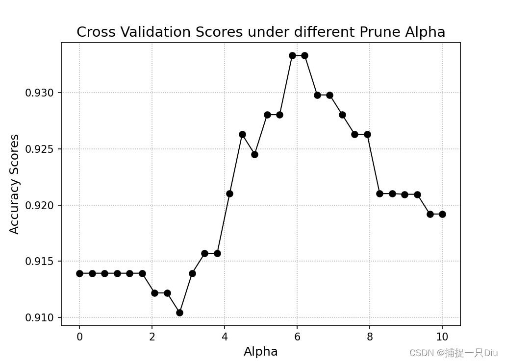
test_decision_tree_C_3.py

import copy
 
import numpy as np
import matplotlib.pyplot as plt
from decision_tree_C import DecisionTreeClassifier
from sklearn.datasets import load_breast_cancer, load_iris
from sklearn.metrics import classification_report, accuracy_score
from utils.plt_decision_function import plot_decision_function
from sklearn.model_selection import StratifiedKFold
 
 
bc_data = load_breast_cancer()
X, y = bc_data.data, bc_data.target
alphas = np.linspace(0, 10, 30)
accuracy_scores = []  # 存储每个alpha阈值下的交叉验证均分
cart = DecisionTreeClassifier(criterion="cart", is_feature_all_R=True, max_bins=10)
for alpha in alphas:
    scores = []
    k_fold = StratifiedKFold(n_splits=10).split(X, y)
    for train_idx, test_idx in k_fold:
        tree = copy.deepcopy(cart)
        tree.fit(X[train_idx], y[train_idx])
        tree.prune(alpha=alpha)
        y_test_pred = tree.predict(X[test_idx])
        scores.append(accuracy_score(y[test_idx], y_test_pred))
        del tree
    print(alpha, ":", np.mean(scores))
    accuracy_scores.append(np.mean(scores))
 
plt.figure(figsize=(7, 5))
plt.plot(alphas, accuracy_scores, "ko-", lw=1)
plt.grid(ls=":")
plt.xlabel("Alpha", fontdict={"fontsize": 12})
plt.ylabel("Accuracy Scores", fontdict={"fontsize": 12})
plt.title("Cross Validation Scores under different Prune Alpha", fontdict={"fontsize": 14})
plt.show()