TensorFlow 常用类与方法_tensorflow.contrib.framework.python.ops import add

简述

Google开源, 算是最早(2016前后)流行的通用, 出圈的 ML 框架.
API 快速参考点 这里.
国内环境可以访问 google 的cn站点, 点 这里。

一. graph 与 session

graph 与 session, 前者是静态的神经网络计算图; 后者是有数据流动的动态计算. 好比 程序与进程 的关系, 也好比 河道与水流 的关系.

1.1 Graph

Graph=(Node,Edge), 前者叫 operation ,负责产生与计算 tensor; 后者就是 tensor 在 nodes 间的流动.

• class tensorflow.python.framework.ops.Graph
  • _collections, 字段. 是一个 Dict [ str, List[ tf.Variable | tf.Tensor | tf.Operation] ], 是对不同 tensor 的聚合与隔离, 详见下文.
  • get_collection_ref(self, name), 根据 name 从 _collections dict 中找对应 list 对象作返回.
  • get_operations(), 可以列出一个 graph 中所包含的所有op. op对象含有丰富的 fields, 可以解析它的输入与输出.

常用的 key 有:

• variables, 计算图中的 + batchNorm的 + optimizer的 各种 tensor
• trainable_variables, 计算图中的 + batchNorm的 各种 tensor
• update_ops,通常为 <tf.Tensor ‘scope_yichu/scope_yichu/BatchNorm/cond_1/Merge:0’ shape=(1,) dtype=float32> 等
• global_step, 通常为 [<tf.Variable ‘global_step:0’ shape=() dtype=int64_ref>]
  - train_op, 通常为 [<tf.Operation ‘OptimizeLoss/train’ type=AssignAdd>]

GraphKeys 这个类定义了一些静态字段与之对应:

• GLOBAL_VARIABLES = “variables”
• LOCAL_VARIABLES = “local_variables”
• TRAINABLE_VARIABLES = “trainable_variables”

不显式地创建 graph 时， 系统会自动创建一个默认的 graph object，该对象可以通过 tf.get_default_graph() 获得.

# 验证默认的 graph
c = tf.constant(4.0)
assert c.graph is tf.get_default_graph()

# 也可以显式地自己创建
g = tf.Graph()
with g.as_default():
  # Define operations and tensors in `g`.
  c = tf.constant(30.0)
  assert c.graph is g
1
2
3
4
5
6
7
8
9
10

1.2 variable_scope 与 context

py 编程中, 定位一个变量, 需要 包名->对象名->字段名, tf 计算图中也会有很多的变量, 怎么定位呢? 它也有自己的完全限定名.
通常通过 variable_scope 设计来隔离与区分, 使用效果见下:

whih tf.variable_scope('aa') as aa:
	a = tf.constant(name='a', value=[1])
	vs2 = tf.variable_scope('bb')
	vs2.__enter__()
	b = tf.constant(name='b', value=[1])
print("a,b", a, b)
1
2
3
4
5
6

Q: 原理是什么呢?
A: variable_scope 是一个类, 位于 tensorflow.python.ops.variable_scope.variable_scope , 构造函数的必填参数为 name_or_scope.
with 语句等价于构造对象后调用 __enter__() 方法, 它会拿到关联的 graph 对象, 并将当前 name 拼接到 graph._name_stack 中.
当调用 tf.get_variable(name) 时, 也会拿到关联的 graph 对象, 将 graph._name_stack与当前 name 拼接, 作为创建对象的完全限定名.

1.3 arg_scope

• tensorflow.contrib.framework.python.ops.arg_scope.arg_scope(list_ops_or_scope, **kwargs)
  将共性的参数提前集中声明, 可以让代码更简洁紧凑.

  with arg_scope([layers.fully_connected, layers.conv2d],
	  weights_initializer='xavier_initializer',
	  weights_regularizer=nn.l2_loss,
	  biases_initializer=init_ops.zeros_initializer()
	  ):
	    net1 = layers.conv2d(net, 256, [5, 5], scope='conv2')
	    net2 = layers.dense(net, 100)
# 这样写, api 的 weights_initializer, weights_regularizer 等参数就会自动对应上 arg_scope 中提前设定好的那些.
1
2
3
4
5
6
7
8

1.4 Session 与 initializer

在 graph 启动之前, 所有的 var 都可以看作 placeholder, 并没有实际, 具体的值去填充. 所以 session 就是一个让 graph launch 起来的机制.

• tensorflow.python.client.session.BaseSession.run(self, fetches, feed_dict=None, options=None, run_metadata=None)
  执行算子 与 计算 tensor 的值. 对于当次传入的 fetches, tf 只会运行计算图中的 necessary graph fragment. 意味着分类任务中, fetch=get_logits 与 fetch=get_loss 所需的最小计算子图是不一样的.
  • fetches, 可以是单个元素或一个 list 或一个 dict. 元素可以是 {tf.Operation, tf.Tensor, tf.SparseTensor} 等.
    每个元素也可以是集合类型, 如 fetches=[op1, {'a':op2}, [op3,op4], tf_var], 足够灵活.
  • feed_dict, Dict[placeholder, 原生的python类型数值 ]
  • Returns, 与 fetches 对应, a single value or a list of values. 有些 train_op 这样的 fetch 元素是没有具体返回值的, 但位置还在.

创建 session 后, 通用流程是:

1. 对 tensor 的权重作初始化填充. 在 tf.get_variable(initializer=None) 这样的api中,
2. 一个 while 循环, 逐个 step 的喂数据做训练.

• tf.global_variables_initializer()
  Returns an Op that initializes global variables. 内部调用了 variables.py 中的 variables_initializer(var_list=global_variables()), 该 Op runs all the initializers of the variables in var_list in parallel.

二. tensor

可分为多种, 如 模型的首层输入tensor, 计算得到的tensor, 构建的常量tensor, 及参与训练的 trainable tensor.

2.1 placeholder

tf.placeholder(dtype, shape=None, name=None)
占位符. 通常用于输入与输出, 即features与labels.
一个例子
x = tf.placeholder(tf.float32, shape=(number_of_samples, INPUT_DIMENSION), name="x-input")

TIPS: 这里的shape可以填shape=(None, INPUT_DIMENSION) 表示是动态的, 以输入的数据为准. 这样有什么好处呢?
可以指定 batch_size 分批训练, 可以在测试集中使用与训练集不同的 batch_size 来评价.

2.2 variable

• tf.Variable
  类. 表示tf中可以被训练的变量. 比如网络层之间的连接权重.
  __init__(self, initial_value=None, ... , name=None, ...)
  必须指定初始值, 起个名字方便在tf-board中看.

• tf.get_variable(name,shape,dtype,initializer=None,...)
  既可以创建 variable, 也可以复用之前创建的 variable.

  • initializer: 常见的有 tf.zeros_initializer. 当发现参数为 None, 则默认使用 tf.glorot_uniform_initializer. 也可以通过tensor来指定, 如other_variable = tf.get_variable("other_variable", dtype=tf.int32, initializer=tf.constant([23, 42])).
  • 这里的 initializer 只是声明, 只有 session.run(tf.global_variables_initializer()) 时, 才会执行此处指定的 initializer.

import tensorflow as tf
a=tf.get_variable(name='a',shape=[2, 3],initializer=tf.truncated_normal_initializer)
a1 = tf.get_variable(name='a', shape=[2, 3], initializer=tf.truncated_normal_initializer)
"""
ValueError: Variable a already exists, disallowed. Did you mean to set reuse=True or reuse=tf.AUTO_REUSE in VarScope? Originally defined at: xxx
"""
1
2
3
4
5
6

2.3 constant

todo.

2.4 Initializer

为了配合 tf.get_variable(), tf提供了常用的 initializer.

• tf.constant_initializer
• tf.random_normal_initializer
• tf.random_uniform_initializer
• tf.zeros_initializer
• tf.ones_initializer
• tf.truncated_normal_initializer
  即classTruncatedNormal(Initializer), 构造函数为def __init__(self, mean=0.0, stddev=1.0, seed=None, dtype=dtypes.float32)
  初始化为满足正态分布的随机值, 但如果一个值偏离平均值超过两个标准差, 会被舍弃重新生成.
• xavier_initializer

This initializer is designed to keep the scale of the gradients roughly the
same in all layers. In uniform distribution this ends up being the range:
x = sqrt(6. / (in + out)); [-x, x] and for normal distribution a standard
deviation of sqrt(2. / (in + out)) is used.

random_seed: 给 Initializer用的随机数种子. 如果不设, 随机数种子也被随机生成, 意味着每次from scratch训练时, 参数的初始值也不同.
可通过tf.estimator.RunConfig(tf_random_seed=21) 设置, 这样更容易复现前一次的结果.

• tf.global_variables_initializer()
  返回一个op (operation), 表示初始化 tf.GraphKeys.GLOBAL_VARIABLES collection 中的所有变量.
  需要注意的是, 这个操作的位置不能随意放, 必须在计算图搭建完成之后调用!

2.6 reset

tf.reset_default_graph() , 重置当前的张量图, 相当于清空所有的张量, 在 jupyter 中可以用到, 比如有些cell 执行过后不满意,就可抹掉执行效果.

三. 运算操作(op)

3.1 tensor生成

• tensorflow.python.ops.random_ops.truncated_normal(shape, mean=0.0, stddev=1.0, dtype=dtypes.float32, seed=None, name=None)
  truncated normal distribution. 初始化为满足正态分布的随机值, 但如果一个值偏离平均值超过两个标准差, 会被舍弃重新生成.
  可通过tf.truncated_normal()调用.

• tensorflow.python.ops.random_ops.random_uniform(shape, minval=0, maxval=None, dtype=dtypes.float32, seed=None, name=None)
  均匀分布, 可通过 tf.random_uniform() 调用.

• tf.ones(shape)
  生成全1的tensor.

• tf.ones_like(tensor,...)
  Creates a tensor with all elements set to 1. type and shape are same of tensor.

• tf.one_hot(indices, depth, ...)
  指定 index 与 depth, 返回一个 one-hot tensor. 例子:

sess.run(tf.one_hot(2, 3)) # [0,0,1]
sess.run(tf.one_hot(0, 3)) # [1,0,0]
1
2

3.2 tensor 转换

• tf.expand_dims(input, axis=None, name=None, dim=None)
  即tensorflow.python.ops.array_ops.expand_dims(...) 方法. 在给定的input这个tensor中增加一维.
  axis: 要向 input 中插入的轴. 若为-1, 表示追加在末尾.
• tf.squeeze(input,axis=None,...)
  降维. 将size为1的那些维度给降掉. 例子见下:

# 't' is a tensor of shape [1, 2, 1, 3, 1, 1]
tf.shape(tf.squeeze(t))  # [2, 3]
1
2

• tf.cast(x, dtype, name=None)
  即 Casts a tensor to a new type. 如将tf.feature_column.input_layer(...)返回的tf.float类型转换为tf.int类型.

• tf.reshape(tensor, shape, name=None)
  用于改变一个tensor的形状. 类似于 np.reshape(). 例子:

t=[1, 2, 3, 4, 5, 6, 7, 8, 9]
reshape(t, [3, 3]) ==> [[1, 2, 3],
                          [4, 5, 6],
                          [7, 8, 9]]
1
2
3
4

• tf.tile(input, multiples, ...):
  Constructs a tensor by tiling a given tensor. 即重复拼接.

3.3 常用运算

Q1:同样的layer处理, 有时既有class又有对应的function interface, 如tf.layers.Conv2D与tf.layers.conv2d, 有什么区别呢?
A: 这些class继承自tensorflow.python.layers.base.Layer, 基类实现了__call__(self, inputs, *args, **kwargs)的方法, 就是该类的对象就变成了可调用对象, 后面可以直接传参数inputs, 便于网络中引出分支或多个input使用同样的layer进行数据传递.

Q2: 我们在使用tensorflow时，会发现tf.nn，tf.layers， tf.contrib模块有很多功能是重复的, 尤其是卷积操作,怎么区别与联系?
A:下面是对三个模块的简述：

1. tf.nn ：提供神经网络相关操作的支持，包括卷积操作（conv）、池化操作（pooling）、归一化、loss、分类操作、embedding、RNN、Evaluation。
2. tf.layers：主要提供的高层的神经网络，主要和卷积相关的，个人感觉是对tf.nn的进一步封装，tf.nn会更底层一些。
3. tf.contrib：tf.contrib.layers提供够将计算图中的 网络层、正则化、摘要操作、是构建计算图的高级操作，但是tf.contrib包含不稳定和实验代码，有可能以后API会改变。

以上三个模块的封装程度是逐个递进的。

单个 tensor

• tf.split(value, num_or_size_splits, axis=0,...)
  对 tensor 进行切分. For example:

  # 'value' is a tensor with shape [5, 30]
  # Split 'value' into 3 tensors with sizes [4, 15, 11] along dimension 1
  split0, split1, split2 = tf.split(value, [4, 15, 11], 1)
  tf.shape(split0)  # [5, 4]
  tf.shape(split1)  # [5, 15]
  tf.shape(split2)  # [5, 11]
  # Split 'value' into 3 tensors along dimension 1
  split0, split1, split2 = tf.split(value, num_or_size_splits=3, axis=1)
  tf.shape(split0)  # [5, 10]
  1
  2
  3
  4
  5
  6
  7
  8
  9

• tf.gather(params, indices,...)
  用于抽取一个tensor中的不连续的slice.

x = np.array([[1] * 5, [2] * 5, [3] * 5])
print('x=', x)
y = tf.gather(x, indices=[0, 2])
print('y=', y)
"""
x= [[1 1 1 1 1]
 [2 2 2 2 2]
 [3 3 3 3 3]]
y= tf.Tensor(
[[1 1 1 1 1]
 [3 3 3 3 3]], shape=(2, 5), dtype=int32)
"""
1
2
3
4
5
6
7
8
9
10
11
12

• tf.reshape(tensor, shape, name=None)
  跟numpy类似, -1表示自动推断, 第一维要考虑到 batch_size, 这是与 keras 的 reshape 有区别的地方.
  Args:

  • shape
    如果 tensor 的 shape 为[1,], 那么shape=[] , 表示要把 tensor 转换成为一个 scalar. 这是与np.reshape()不同的地方, np 不接受[]这样的参数.

• tf.layers.flatten(inputs, name=None)
  将tensor展开为(BATCH_SIZE,展开后的维度)的一维形式.

• tf.square(x, name=None), 计算平方.

• tf.sqrt(x, name=None) , square_root, 计算平方根.

• tf.reduce_mean(input_tensor,axis=None)
  Reduces input_tensor along the dimensions given in axis

• tf.reduce_sum(input_tensor,axis=None,...)
  Computes the sum of elements across dimensions of a tensor.

x = tf.constant([[1, 1, 1], [1, 1, 1]])
tf.reduce_sum(x)  # 6
tf.reduce_sum(x, 0)  # [2, 2, 2]
tf.reduce_sum(x, 1)  # [3, 3]
1
2
3
4

• tf.stop_gradient(input)
  Prevents the contribution of its inputs to be taken into account when compute gradients.

emb/卷积/池化类

• tf.nn.embedding_lookup(params,ids, partition_strategy="mod", name=None, ...)
  方法, 快速查找id对应的张量.
  params: 即 embedding_matrix.
  ids: A Tensor with type int32 or int64 containing the ids to be looked up in params.
• tf.layers.conv2d(inputs,filters,kernel_size,strides=(1, 1), padding='valid',...)
  二维卷积, inputs.shape 需要为None,x,x,x这样的四维结构.
• tf.layers.max_pooling2d((inputs,pool_size, strides,...)
  配合 conv2d 使用,

同层之间的运算

• tf.tensordot(a, b, axes, name=None)
  两个 tensor 之间的 点乘, 即 dot product. 此方法没搞懂, 慎用. 想求点乘还是用熟悉的 tf.reduce_sum(tf.multiply(a, b), axis=1) 较好.
• tf.multiply(a,b)
  等同于np的数组乘法, 即对应元素相乘.
• tf.keras.layers.dot(inputs, axes, normalize=False)
  keras的点乘操作, normalize=True 就等价于 cosine similarity.

前后层之间的运算

• tf.layers.dense(inputs,units,activation=None,use_bias=True,...)
  增加一层全连接. 返回计算后的tensor. 需要的 W,b及激活层都会被自动的创建.
• tf.contrib.layers.fully_connected(inputs, num_outputs, activation_fn=nn.relu, ...)
  与tf.layers.dense 功能相同.
• tf.matmul(a,b)
  Multiplies matrix a by matrix b.
• tf.nn.xw_plus_b(x, weights, biases, name=None)
  常用操作的封装, Computes matmul(x, weights) + biases.
  Args:
  x: a 2D tensor. Dimensions typically: batch, in_units
  weights: a 2D tensor. Dimensions typically: in_units, out_units
  biases: a 1D tensor. Dimensions: out_units
• tf.nn.softmax(logits, dim=-1, name=None)
  即tensorflow.python.ops.nn_ops.softmax(logits, dim=-1, name=None)
  计算 softmax 激活.

op 之间的依赖与聚合

• tensorflow.python.framework.ops.control_dependencies(control_inputs)
  Returns a context manager. All operations constructed within the context, 都会被确保在 control_inputs 得到执行后再执行.
  使用场景是 BatchNorm 参数先更新, optimizer 的 train_op 再执行.
• tensorflow.python.ops.control_flow_ops.group(*inputs, **kwargs)
  An Operation that executes all its inputs.

四. 条件语句

python中可以自然地写 if,switch 等条件语句. 但静态图不能, 只能借助以下几个方法实现.

• tf.cond(pred,true_fn,false_fn)
  Return true_fn() if the predicate pred is true else false_fn().
• tf.greater(x,y)
  Returns the boolean value of whether (x > y) element-wise
• tf.where(condition,x,y)
  两种用法.
  1. x,y 都为None, 此时返回的是 True 值的index, 注意 shape=(${true_cnt}, ) 为不定长
  2. x,y 均有值且shape均与condition一致. 此时 相当于条件函数, 对应位置若为True, 返回x相应位置的值, 否则返回y相应位置的值.
• tf.case({谓词1:fn_1, 谓词2:fn_2, 谓词3:fn_3})
  fn 这里有要求, 返回值必须是 tensor. 该 api 的签名中, 不让给 fn 传参. 解决思路是用 lambda/闭包 语法, 变相实现传参.

4.2 例子

t = [1, 1, 0, 1]
cond = tf.greater(t, 0)
print('cond=', cond)
where_1_index = tf.where(cond)[:, 0]
print('where_1_index=', where_1_index)
where_2_elements = tf.where(cond, [88] * 4, [99] * 4)
print('where_2_elements=', where_2_elements)
"""
cond= tf.Tensor([ True  True False  True], shape=(4,), dtype=bool)
where_1_index= tf.Tensor([0 1 3], shape=(3,), dtype=int64)
where_2_elements= tf.Tensor([88 88 99 88], shape=(4,), dtype=int32)
"""
1
2
3
4
5
6
7
8
9
10
11
12

五. loss 损失函数

详见参考[1] .

六. gradient 与 optimizer

详见参考[5].

七. 动态配置

为了让程序中的超参数更灵活, 采用配置文件的方式. 同 java 中的 .properties 文件如出一辙.
在tf中可以这么写 :

import tensorflow as tf  

FLAGS = tf.app.flags.FLAGS

#表示从配置文件中读取learning_rate变量的值, 如果读不到以 0.01 作默认值. 注解为 "学习速率".
#类似地, 还有 `DEFINE_integer()`, `DEFINE_boolean()`等.
tf.app.flags.DEFINE_string("learning_rate", "0.01", "learning rate")

FLAGS = tf.app.flags.FLAGS 
#读出来配置的值
learning_rate=FLAGS.learning_rate
1
2
3
4
5
6
7
8
9
10
11

八 . tf.metrics 评估指标

eval 通常与 train 并行, 此时就可以计算评估指标.
它们一般都会用到 local variable, 对应 tf.GraphKeys.LOCAL_VARIABLES .

8.1 accuracy 准确率

• tf.metrics.accuracy(labels, predictions, …)
  计算准确率, 即 labels与predictions 相一致的频率. 内部维护了两个 local variable, count 与 total, $accuracy=\frac{count}{total}$. 所以这个适用于 stream data 的数据评估.
  注意它的返回参数有两个, 第一个是当前的准确度tensor, 第二个是更新 total 与 count 的op, 对这个op的run, 返回的是这次调用后的最新准确度.
  用法示例见 : Stack Overflow 讨论

8.1 auc

分类问题常用auc.

• tf.metrics.auc(labels,predictions, curve=‘ROC’,…)
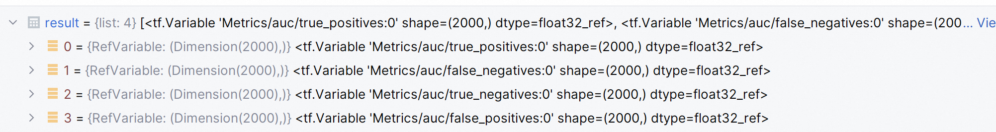
  该方法会创建四个本地变量, {true_positives,
  true_negatives, false_positives and false_negatives}, 辅助计算 auc.
  该方法可以流式计算 auc (streaming_auc).
  • num_thresholds, 离散的点越多, auc 预估就越准确
  • returns:
    • auc, a scalar Tensor.
    • update_op, 相应地更新四个本地变量. 感觉没说清楚, 可以当 totoal_auc.

九. Layer 与 Keras

详见参考[4]

参考

1. my blog， 常用损失函数及tf实现
2. my blog, TensorFlow RNN 相关类与方法
3. my blog, 机器学习中的正则项及梯度截断
4. my blog, tf与keras中的layer
5. my blog, tensorflow 中的 gradient 与 optimizer