ViT（ Vision Transformer）详解

（一）参考博客和PPT原文件下载连接

首先感谢一下各位博主写的优秀文章供我们参考。

• (知乎)详解Transformer （Attention Is All You Need）
• 多头注意力机制
• Vision Transformer详解

链接： 李宏毅老师self-attention和本文中用到的PPT下载
提取码：p63y
–来自百度网盘超级会员V4的分享

（二）VIT原理详解

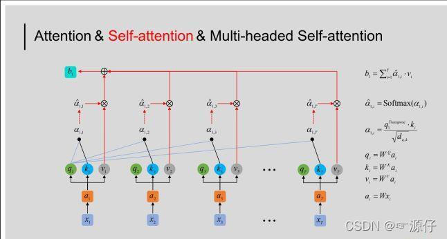
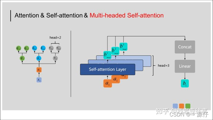
我们首先看一下Self-Attention的整体计算过程的结构图：（此图片来源于Multi-headed Self-attention（多头自注意力）机制介绍）。

2.1、self-attention

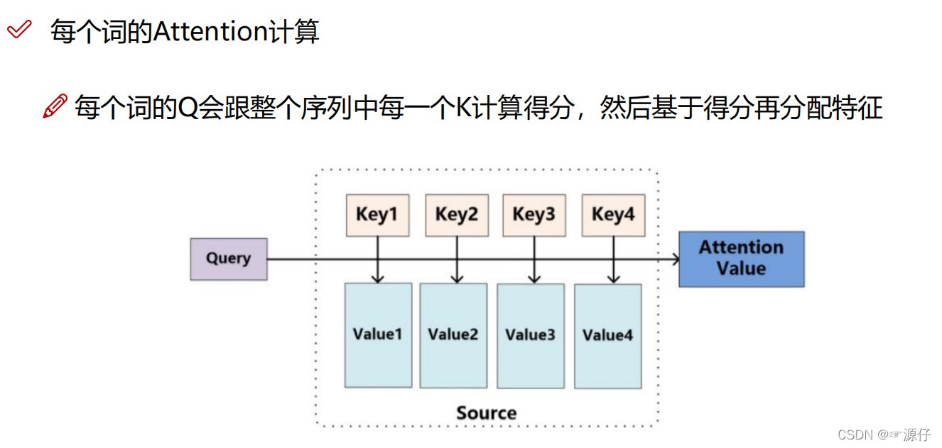
首先我们看 图1，attention是啥意思？

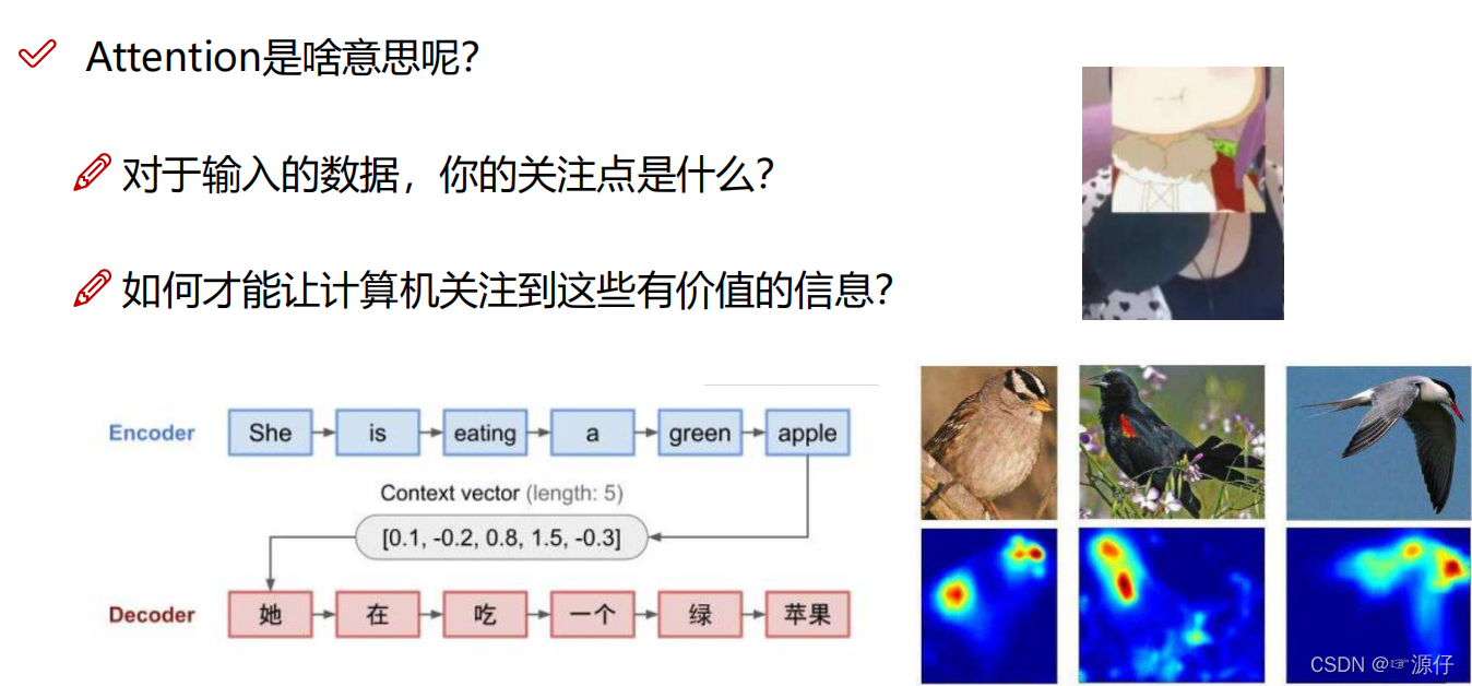
            图1 、什么是attention
2、Transformer的整体框架 图2 所示：

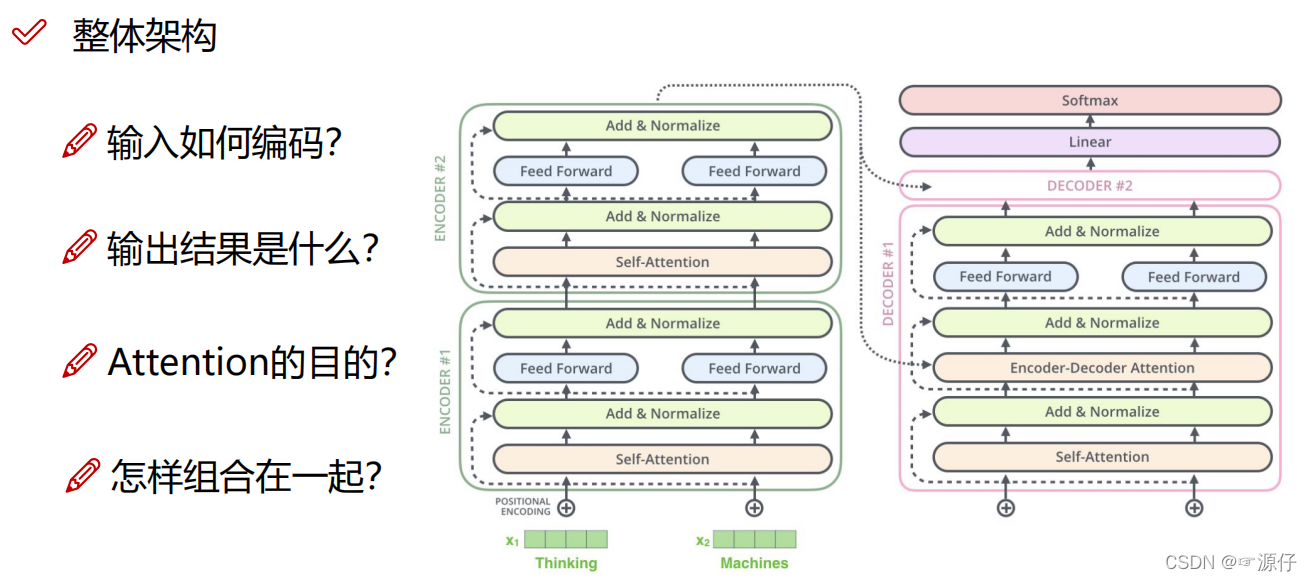
            图2、Transformer的整体框架

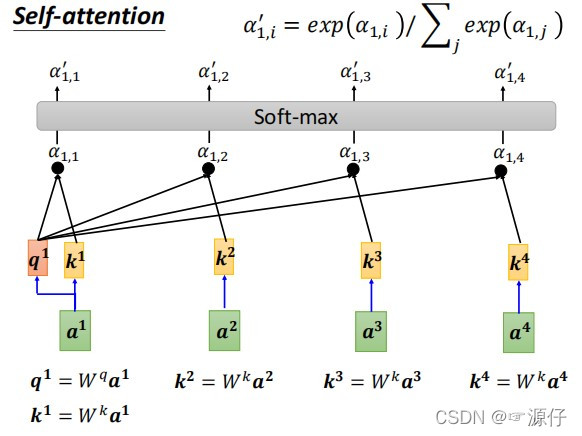
3、self-attention是怎样计算的。如图3 所示：

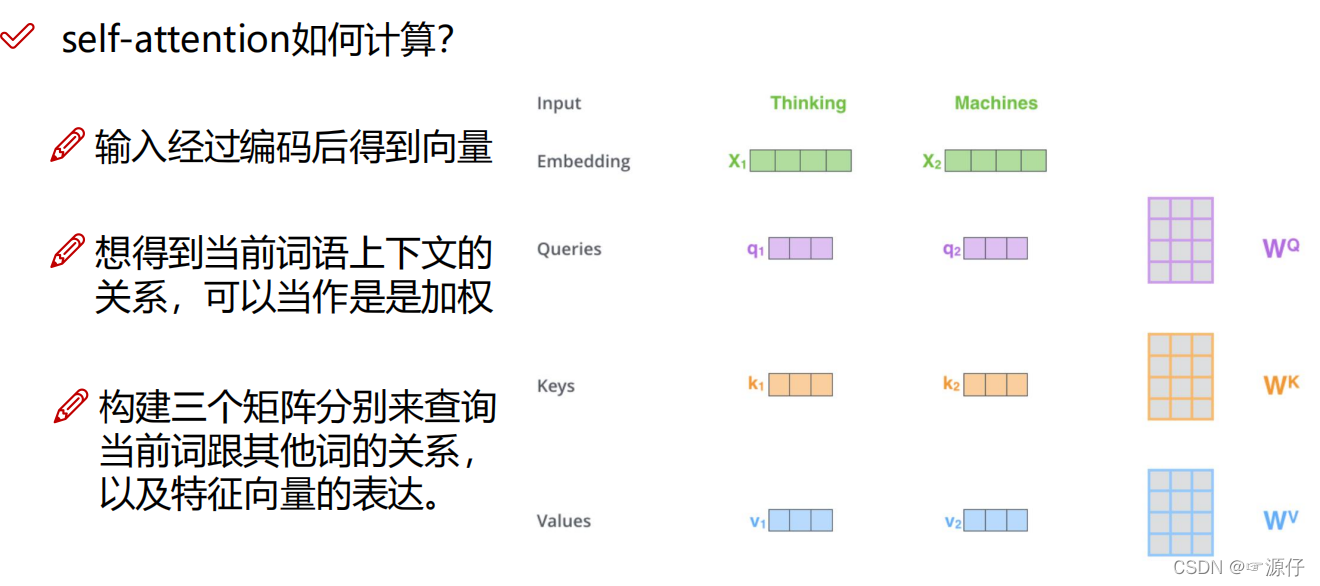
           图3、self-attention是怎样计算的？
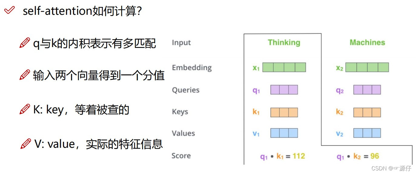
4、首先我们要知道三个参数量的名称和大概的作用：如图4：

• Q : query（查询）：我们要去查询什么东西
• K ： Key（关键）：指被查询的东西
• V ：value(值) ：指的是对实际输入信息的提取的特征信息（大概和CNN中提取Feature Map的含义差不多）。
  

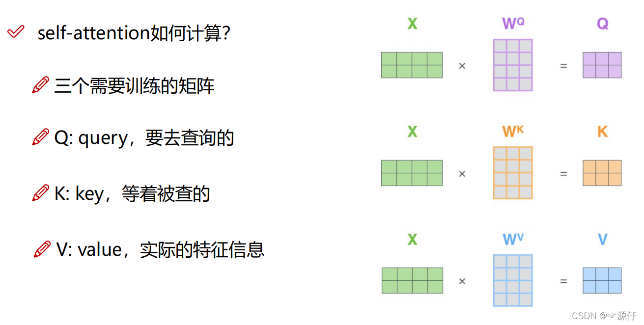
           图4、Q、K、V的含义

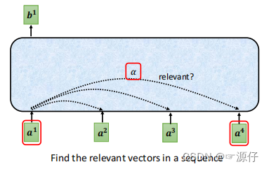
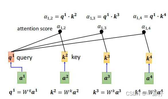
2.2、sequence序列之间相关性$\mathbf{\alpha }$的求解

sequence序列之间相关性的求解：相关性用$\mathbf{\alpha }$表示。因为self-attention的特点就是具有全局性，但是拥有全局性，必须使每个序列之间都要有关联。如下图5所示：

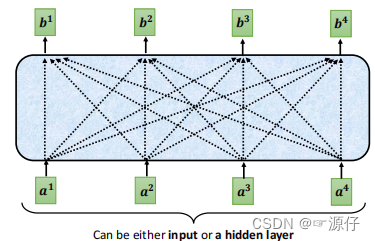
           图5、全局性的表达
  图5中是不是和全连接层很像，中间的是隐层，也就是权重$W$。但是我们好像不能按照上面图5这样直接连接吧，不然$a^1$，$a^2$，…，$a^4$之间的相关性都一样，没有任何区别，那么输出的$b^1$，$b^2$，…，$b^4$那不就都一样了哈。所以我们要计算$a^1$，$a^2$，…，$a^4$之间的相关性$\mathbf{\alpha }$。
  我们先看图，好理解：


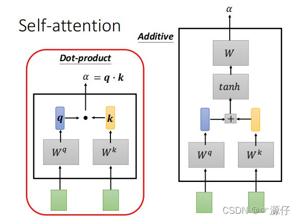
为什么上面用Dot-Product去计算相关性$\mathbf{\alpha }$呢？
  向量的点乘可以用来计算两个向量之间的夹角，进一步判断这两个向量是否正交（垂直）等方向关系。 同时，还可以用来计算一个向量在另一个向量方向上的投影长度。
  那么当两个向量的夹角为$90^{\circ }$时，Dot-Product的结果为0，这里表示相关性为0；当两个向量重合或平行时，Dot-Product的结果为无穷大，想一想当两个向量平行时，是不是代表这两个向量之间是不是成比例关系，那这两个向量是不是相似（即指这里的相关性），所以当点乘之间的结果越大，他们的相关性越强。

下面我们看一下用矩阵表示时候的计算过程图吧：

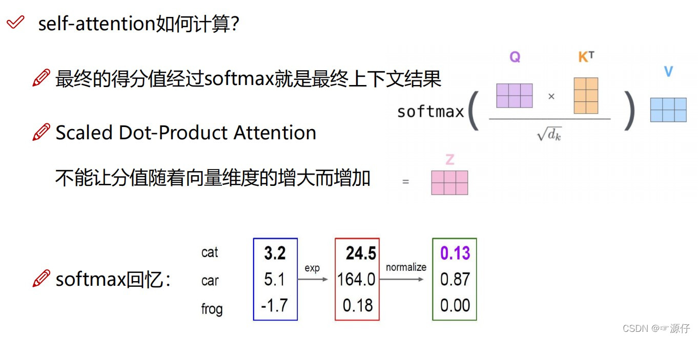
由上图我们可以注意到一个公式：
$Attention(Q,K,V)=softmax(\frac{Q{K}^T}{\sqrt{d_k}})V=softmax(\frac{\mathbf{\alpha }}{\sqrt{d_k}})V$:

除以$\sqrt{d_k}$的作用：

  如果Dot-Product点乘的结果很小，Additive Attention 和 Dot-Product-Attention的效果差不多。
  如果Dot-Product点乘的结果很大，如果不除以$\sqrt{d_k}$做Scaling，那么结果就不如Additive Attention。
  此外，点乘结果过大，在进行Softmax之后的梯度会变得很小，不利于反向传播。

2.3、Value与相关性$\mathbf{\alpha }$之间的计算

2.4、多头注意力机制

在Transformer及BERT模型中用到的Multi-headed Self-attention结构与之略有差异，具体体现在：如果将前文中得到的$q_i,k_i,v_i$,整体看做一个“头”，则“多头”即指对于特定的 $x_i$来说，需要用多组$W^Q,W^K,W^V$与之相乘，进而得到多组$q_i,k_i,v_i$。如下图所示：

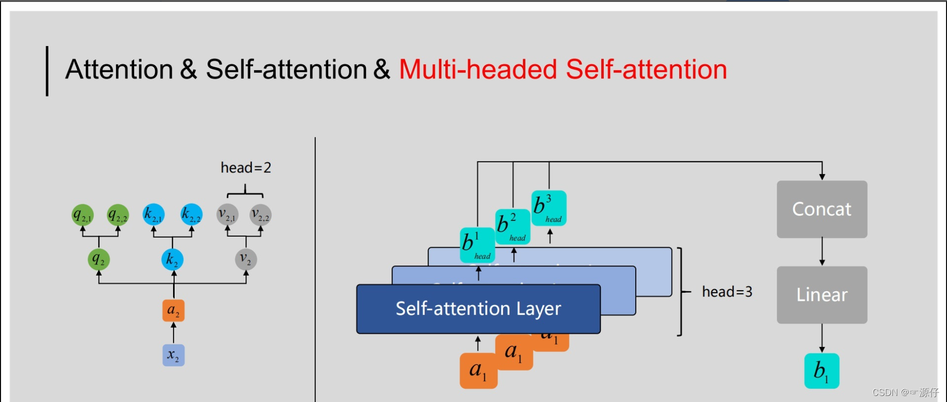
如上图所示，以右侧示意图中输入的 $a_1$为例，通过多头（这里取head=3）机制得到了三个输出 $b_{head}^1,b_{head}^2,b_{head}^3$,为了获得与 $a_1$对应的输出$b_1$，在Multi-headed Self-attention中，我们会将这里得到的$b_{head}^1,b_{head}^2,b_{head}^3$进行拼接（向量首尾相连），然后通过线性转换（即不含非线性激活层的单层全连接神经网络）得到$b_1$。对于序列中的其他输入也是同样的处理过程，且它们共享这些网络的参数。

（三）Transformer代码详解

(1)、VIT 的 总的前向传播代码：

class VisionTransformer(nn.Module):
    def __init__(self, config, img_size=224, num_classes=21843, zero_head=False, vis=False):
        super(VisionTransformer, self).__init__()
        self.num_classes = num_classes
        self.zero_head = zero_head
        self.classifier = config.classifier

        self.transformer = Transformer(config, img_size, vis)
        self.head = Linear(config.hidden_size, num_classes)

    def forward(self, x, labels=None):
        x, attn_weights = self.transformer(x)
        print(x.shape)
        logits = self.head(x[:, 0])  # x[:, 0]=(16,768) :16是batch_size,789是197个tokens的维度，这里是取是第0个token，也就是那个用于分类的token
        print(logits.shape)

        if labels is not None:
            loss_fct = CrossEntropyLoss()
            loss = loss_fct(logits.view(-1, self.num_classes), labels.view(-1))
            return loss
        else:
            return logits, attn_weights
1
2
3
4
5
6
7
8
9
10
11
12
13
14
15
16
17
18
19
20
21
22

如下会类Transformer代码中Embeddings和Encoder两个定义结合结果图讲解。

class Transformer(nn.Module):
    def __init__(self, config, img_size, vis):
        super(Transformer, self).__init__()
        self.embeddings = Embeddings(config, img_size=img_size)
        self.encoder = Encoder(config, vis)

    def forward(self, input_ids):
        embedding_output = self.embeddings(input_ids)
        encoded, attn_weights = self.encoder(embedding_output)
        return encoded, attn_weights
1
2
3
4
5
6
7
8
9
10

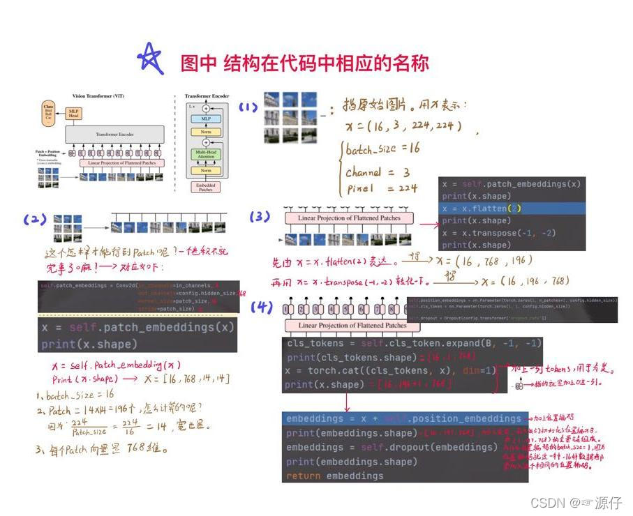
3.1、Transformer中Embeddings类的讲解

class Embeddings(nn.Module):
    """Construct the embeddings from patch, position embeddings.
    """
    def __init__(self, config, img_size, in_channels=3):
        super(Embeddings, self).__init__()
        self.hybrid = None
        img_size = _pair(img_size)

        if config.patches.get("grid") is not None:
            grid_size = config.patches["grid"]
            patch_size = (img_size[0] // 16 // grid_size[0], img_size[1] // 16 // grid_size[1])
            n_patches = (img_size[0] // 16) * (img_size[1] // 16)
            self.hybrid = True
        else:
            patch_size = _pair(config.patches["size"])
            n_patches = (img_size[0] // patch_size[0]) * (img_size[1] // patch_size[1])
            self.hybrid = False

        if self.hybrid:
            self.hybrid_model = ResNetV2(block_units=config.resnet.num_layers,
                                         width_factor=config.resnet.width_factor)
            in_channels = self.hybrid_model.width * 16
        self.patch_embeddings = Conv2d(in_channels=in_channels,
                                       out_channels=config.hidden_size,
                                       kernel_size=patch_size,
                                       stride=patch_size)
        self.position_embeddings = nn.Parameter(torch.zeros(1, n_patches+1, config.hidden_size))
        self.cls_token = nn.Parameter(torch.zeros(1, 1, config.hidden_size))

        self.dropout = Dropout(config.transformer["dropout_rate"])

    def forward(self, x):
        print(x.shape)   # 数据集的图片尺寸(16，3，224，224)，Batch_size = 16
        B = x.shape[0]
        # cls_tokens就是那个单独添加的0的位置，起作用是整合所有序列的特征信息，用于图像分类。
        cls_tokens = self.cls_token.expand(B, -1, -1)
        print(cls_tokens.shape)  # torch.Size([16, 1, 768])
        if self.hybrid:
            x = self.hybrid_model(x)
        x = self.patch_embeddings(x)  # 就是做个卷积，把图像分成指定的patch
        print(x.shape)          # torch.Size([16, 768, 14, 14])
        x = x.flatten(2)        # 把14乘14=196个patch，所以要flatten
        print(x.shape)          # torch.Size([16, 768, 196]) 
        x = x.transpose(-1, -2)
        print(x.shape)          # torch.Size([16, 196, 768])
        x = torch.cat((cls_tokens, x), dim=1) # 整合分类的token
        print(x.shape)          # torch.Size([16, 197, 768])

        embeddings = x + self.position_embeddings
        print(embeddings.shape) # torch.Size([16, 197, 768])
        embeddings = self.dropout(embeddings)
        print(embeddings.shape) # torch.Size([16, 197, 768])
        return embeddings
1
2
3
4
5
6
7
8
9
10
11
12
13
14
15
16
17
18
19
20
21
22
23
24
25
26
27
28
29
30
31
32
33
34
35
36
37
38
39
40
41
42
43
44
45
46
47
48
49
50
51
52
53

3.2、Transformer中Encoder类的讲解

class Encoder(nn.Module):
    def __init__(self, config, vis):
        super(Encoder, self).__init__()
        self.vis = vis
        self.layer = nn.ModuleList()
        self.encoder_norm = LayerNorm(config.hidden_size, eps=1e-6)
        # 定义了多个Block
        for _ in range(config.transformer["num_layers"]):
            layer = Block(config, vis)
            self.layer.append(copy.deepcopy(layer))

    def forward(self, hidden_states):
        print(hidden_states.shape)  # torch.Size([16, 197, 768])，继承Embeddings类的输出维度
        attn_weights = []
        for layer_block in self.layer:
            hidden_states, weights = layer_block(hidden_states)
            if self.vis:
                attn_weights.append(weights)
        encoded = self.encoder_norm(hidden_states)
        return encoded, attn_weights
1
2
3
4
5
6
7
8
9
10
11
12
13
14
15
16
17
18
19
20

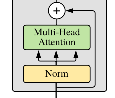
• （1）以下for循环代码是指形成L个Transformer Encoder Block结构，如下图所示

# 定义了L个Block，如下图
        for _ in range(config.transformer["num_layers"]):
            layer = Block(config, vis)
            self.layer.append(copy.deepcopy(layer))
1
2
3
4

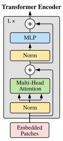
3.2.1、Encoder类中的Block类(拼图学习法)

• （2）查看Encoder类中的Block类：是如何定义的。

class Block(nn.Module):
    def __init__(self, config, vis):
        super(Block, self).__init__()
        self.hidden_size = config.hidden_size
        self.attention_norm = LayerNorm(config.hidden_size, eps=1e-6)
        self.ffn_norm = LayerNorm(config.hidden_size, eps=1e-6)
        self.ffn = Mlp(config)  # 就是一系列全连接操作
        self.attn = Attention(config, vis)

    def forward(self, x):
        print(x.shape)  # torch.Size([16, 197, 768])
        h = x    # 为了开始的残差连接做准备，后面做加法（x + h）
        x = self.attention_norm(x)
        print(x.shape)  # torch.Size([16, 197, 768])
        x, weights = self.attn(x)
        x = x + h
        print(x.shape)  # torch.Size([16, 197, 768])

        h = x
        x = self.ffn_norm(x)
        print(x.shape)  # torch.Size([16, 197, 768])
        x = self.ffn(x)
        print(x.shape)  # torch.Size([16, 197, 768])
        x = x + h
        print(x.shape)  # torch.Size([16, 197, 768])
        return x, weights
1
2
3
4
5
6
7
8
9
10
11
12
13
14
15
16
17
18
19
20
21
22
23
24
25
26

(1)、这一部分代码如下图所示：

h = x    # 为了开始的残差连接做准备，后面做加法（x + h）
x = self.attention_norm(x)
print(x.shape)  # torch.Size([16, 197, 768])
x, weights = self.attn(x)
x = x + h
1
2
3
4
5

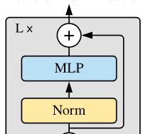
(2)、这一部分代码指的是如下图的结构：

h = x
x = self.ffn_norm(x)
print(x.shape)
x = self.ffn(x)
print(x.shape)
x = x + h
print(x.shape)
return x, weights
1
2
3
4
5
6
7
8

3.2.1.1、Encoder类中的Block类中的Attention类

指的是Block类中的x, weights = self.attn(x)这一行代码，这个attn就是Attention类，这个是重点奥。

class Attention(nn.Module):
    def __init__(self, config, vis):
        super(Attention, self).__init__()
        self.vis = vis
        self.num_attention_heads = config.transformer["num_heads"]
        self.attention_head_size = int(config.hidden_size / self.num_attention_heads)
        self.all_head_size = self.num_attention_heads * self.attention_head_size

        self.query = Linear(config.hidden_size, self.all_head_size)
        self.key = Linear(config.hidden_size, self.all_head_size)
        self.value = Linear(config.hidden_size, self.all_head_size)

        self.out = Linear(config.hidden_size, config.hidden_size)
        self.attn_dropout = Dropout(config.transformer["attention_dropout_rate"])
        self.proj_dropout = Dropout(config.transformer["attention_dropout_rate"])

        self.softmax = Softmax(dim=-1)

    def transpose_for_scores(self, x):
        new_x_shape = x.size()[:-1] + (self.num_attention_heads, self.attention_head_size)
        print(new_x_shape)
        x = x.view(*new_x_shape)
        print(x.shape)
        print(x.permute(0, 2, 1, 3).shape)
        return x.permute(0, 2, 1, 3)

    def forward(self, hidden_states):
        print(hidden_states.shape)  # torch.Size([16, 197, 768])
        # query是一个全连接层，指的是构建Q:查询
        mixed_query_layer = self.query(hidden_states)
        print(mixed_query_layer.shape)  # torch.Size([16, 197, 768])   
        # batch——size = 16，tokens（也可这序列长度） = 197 ，每个tokens都是768维
        # key是一个全连接层，指的是构建K:被查询
        mixed_key_layer = self.key(hidden_states)
        print(mixed_key_layer.shape) # torch.Size([16, 197, 768])
        # value是一个全连接层，指的是构建V:输入的真实特征表达形式
        mixed_value_layer = self.value(hidden_states)
        print(mixed_value_layer.shape) # torch.Size([16, 197, 768])

        query_layer = self.transpose_for_scores(mixed_query_layer) # 详细介绍在3.2.1.1.1、self.transpose_for_scores()
        print(query_layer.shape)
        key_layer = self.transpose_for_scores(mixed_key_layer)
        print(key_layer.shape)
        value_layer = self.transpose_for_scores(mixed_value_layer)
        print(value_layer.shape)

        attention_scores = torch.matmul(query_layer, key_layer.transpose(-1, -2))  # query与key的转置进行点成（也就是self-attention种提到的Dot-Product）。
        print(attention_scores.shape)  # torch.Size([16, 12, 197, 197])
        
        # 这里点乘后为什么变成了[16, 12, 197, 197]，batch_size = 16，attention_head = 12, 那么197和197指什么意思呢
        # 我们知道197指token的数量，又两个向量点乘是指两个向量的相关下程度。
        # 所以这里是指197个tokens分别与自身和其他196个tokens之间的相关程度的大小，也就可以理解为注意力attention的大小。
        attention_scores = attention_scores / math.sqrt(self.attention_head_size)
        print(attention_scores.shape) # torch.Size([16, 12, 197, 197])
        attention_probs = self.softmax(attention_scores)
        print(attention_probs.shape) # torch.Size([16, 12, 197, 197])
        weights = attention_probs if self.vis else None
        attention_probs = self.attn_dropout(attention_probs)
        print(attention_probs.shape)  # torch.Size([16, 12, 197, 197])

        context_layer = torch.matmul(attention_probs, value_layer)  
        # 点乘后得到的[16, 12, 197, 197]与value[16, 12, 197, 64]点乘
        #这一步的意义是用相关性乘以对应提取的输入的特征，这样可以token获取相应具有attention性质的特征。
        print(context_layer.shape)  # torch.Size([16, 12, 197, 64])
        context_layer = context_layer.permute(0, 2, 1, 3).contiguous()
        print(context_layer.shape)  # torch.Size([16, 197, 12, 64])
        new_context_layer_shape = context_layer.size()[:-2] + (self.all_head_size,)
        context_layer = context_layer.view(*new_context_layer_shape)
        print(context_layer.shape)
        attention_output = self.out(context_layer)
        # 还原到输入的形式
        print(attention_output.shape)  # torch.Size([16, 197, 768])
        attention_output = self.proj_dropout(attention_output)
        print(attention_output.shape)  # torch.Size([16, 197, 768])
        return attention_output, weights

1
2
3
4
5
6
7
8
9
10
11
12
13
14
15
16
17
18
19
20
21
22
23
24
25
26
27
28
29
30
31
32
33
34
35
36
37
38
39
40
41
42
43
44
45
46
47
48
49
50
51
52
53
54
55
56
57
58
59
60
61
62
63
64
65
66
67
68
69
70
71
72
73
74
75
76

3.2.1.1.1、self.transpose_for_scores()

把query、key、value转化为多头注意力的size。

size()：函数介绍，不会的简单看一下，浅显易懂。

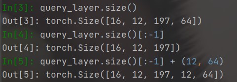
def transpose_for_scores(self, x):
    new_x_shape = x.size()[:-1] + (self.num_attention_heads, self.attention_head_size)  # torch.Size([16, 197, 12, 64])
    print(new_x_shape)
    # 转化为多头注意力机制的size
    x = x.view(*new_x_shape) 
    print(x.shape)         # torch.Size([16, 197, 12, 64])
    print(x.permute(0, 2, 1, 3).shape)
    return x.permute(0, 2, 1, 3)  # torch.Size([16, 12, 197, 64])
1
2
3
4
5
6
7
8

我们记得原始的query是 ([16，197，768]) 的，现在为啥转化为了 ([16, 197, 12, 64]) ，这个12指的是num_attention_heads = 12（多头注意力机制），attention_head_size = 64（注意num_attention_heads的设置一定要被tokens的维度整除，这里tokens的维度维768）。由于在第一节我们详细的讲述了self-attention，所以下面我们看一下多头注意力机制的图片就懂了。每个attention_heads都是单独训练的，就和12个人鸣人会产生12种战斗想法一样，他们是相互独立的。

3.2.2、VIT代码总的前向传播

我们在3.2.1章节中已经详细的讲解了x, attn_weights = self.transformer(x)这一行代码debug的详细过程，那么现在我们再来看VIT总的代码的前向传播就不难理解了。下面我们主要讲解logits = self.head(x[:, 0])这一行代码的作用。
如下图的红色方框部分所示。代那么到此为止，这张图形的所有部分我们都已经用代码按循序凭借完成。所以VIT的主要model代码到此为止，相信大家也完全弄懂了VIT。(1)、VIT 的 总的前向传播代码：

class VisionTransformer(nn.Module):
    def __init__(self, config, img_size=224, num_classes=21843, zero_head=False, vis=False):
        super(VisionTransformer, self).__init__()
        self.num_classes = num_classes
        self.zero_head = zero_head
        self.classifier = config.classifier

        self.transformer = Transformer(config, img_size, vis)
        self.head = Linear(config.hidden_size, num_classes)

    def forward(self, x, labels=None):
        x, attn_weights = self.transformer(x)
        print(x.shape)  # torch.Size([16, 197, 768])
        logits = self.head(x[:, 0])  
        # x[:, 0]=(16,768) :16是batch_size,789是197个tokens的维度，这里是取是第0个token，也就是那个用于分类的token
        # head就是全连接，分类用的。
        print(logits.shape) # torch.Size([12, 10])

        if labels is not None:
            loss_fct = CrossEntropyLoss()
            loss = loss_fct(logits.view(-1, self.num_classes), labels.view(-1))
            return loss
        else:
            return logits, attn_weights
1
2
3
4
5
6
7
8
9
10
11
12
13
14
15
16
17
18
19
20
21
22
23
24