sklearn的系统学习——随机森林分类器与随机森林回归器（含有python完整代码及案例）_sklearn随机森林分类

目录

集成算法

 sklearn中的随机森林

随机森林分类器

随机性参数

属性

案例代码

随机森林回归器

案例代码

---

在前面的内容中，已经对决策树解决分类回归问题分别做了阐述，今天走进随机森林的世界。

什么是森林呢，对，好多树在一起我们就叫它森林，为什么是随机呢，因为这片森林可能不一样，这就涉及到参数的设定了（就像之前决策树的参数一样）。

名字的意义明白了，那这最终的结果是怎么得出来的呢？其实很简单，我们知道一棵决策树会给出一个结果，多棵树就会给出多个结果，最后”投票“表决，得票高的就是最终随机森林给出的结果喽。（当然，这里的解释较为简单，想知道具体原理可以阅读《数据挖掘导论》和西瓜书。）

集成算法

集成学习算法本身不算一种单独的机器学习算法,而是通过构建并结合多个机器学习器来完成学习任务。

目标：集成算法会考虑多个评估器的建模结果，汇总之后得到一个综合的结果，以此获取比单个模型更好的回归或者分类效果。

集成评估器：多个模型集成后的模型，如随机森林。

 分类：bagging（袋装法），boosting（提升法），stacking。主要介绍前两个。

           bagging（袋装法）：模型之间相互独立，互相平行，如随机森林。

           boosting（提升法）：模型之间不相互独立，且模型有序，逐渐提升，如adaboost。

 sklearn中的随机森林

随机森林分类器

参数列表几乎与决策树的相同，重要的有：

criterion,      max_depth,     min_samples_leaf,     min_samples_split,    max_features,   min_impurity_decrease

n_estimators树木的数量，越大往往越好，但达到一定程度之后精确性往往会上下波动，默认10，0.22版本会改为100，一般0-200选一个比较好。

.除此之外，还需要注意的是关于随机性的这两个参数：

随机性参数

1、random_state

当random_state固定时，随机森林中生成的是一组固定的树，但每棵树依然不一致，这是随机挑选特征进行分枝的方法。当随机性越大的时候，袋装法的效果一般会越来越好，用袋装法集成时，基分类器应该是相互独立，是不相同的。

但是局限性强，数据可能没有足够多的特征构建成千上万棵不同的树，因此还需要其他方式。

2、bootstrap & oob_score

使用不同的训练集，袋装法有放回随机抽样技术来形成不同的训练数据，bootstrap就是控制抽样技术的参数。

但是这又会引出如下问题：一些样本可能在同一个自助集出现多次，而其他一些却可能被忽略。一般来说，自助集大约包含63%的原始数据，计算方式：1-（1-1/n)**n，这里是按逆向思维进行计算的：每次都不被选中，总共进行n次，总概率1减去该值即为如上结果。

那既然大约63%的数据被使用，就会有约37%的数据未被使用，这个数据集叫做袋外数据（out of bag data,oob）。除开始划分的测试集，这些也可以用来当测试集——所以，在使用随机森林时，可以不划分测试集和训练集，只需要袋外数据来测试我们的模型即可，当然也不绝对，因为当n和n_estimators都不够大时，很可能就没有数据掉到袋外，自然也就无法使用oob数据来测试模型。

属性

相较决策树，随机森林除feature_importances属性外，

#重要性
importance = clf.feature_importances_
feature_importance = [(feature,importance.round(3)) for feature,importance in zip(feature_name,importance)]
#排序
feature_importance = sorted(feature_importance,key=lambda x :x[1],reverse=True)
#对应进行打印
[print('variable:{:20} importance: {}'.format(*pair)) for pair in feature_importance]

还有如下两个属性：

1、estimators_

#随机森林的重要属性：estimators_,查看森林中树的情况
 
print(rf.estimators_)
 
rf.estimators_[1].random_state

2、 oob_score

rf = RandomForestClassifier(n_estimators=25,random_state=42,oob_score=True)
oob = rf.oob_score_

案例代码

from sklearn.ensemble import RandomForestClassifier
from sklearn.tree import DecisionTreeClassifier
import matplotlib.pyplot as plt
from sklearn.datasets import load_wine
from sklearn.model_selection import train_test_split
from sklearn.model_selection import cross_val_score
 
wine = load_wine() #字典
print(wine.data) #可以通过键取值
print(wine.data.shape)
print(wine.target)
 
xtrain,xtest,ytrain,ytest = train_test_split(wine.data,wine.target,test_size=0.3)
rf = RandomForestClassifier(n_estimators=25,random_state=42,oob_score=True)
clf = DecisionTreeClassifier(random_state=42)
#交叉验证
cross_rf = cross_val_score(rf,wine.data,wine.target,cv=5)
cross_clf = cross_val_score(clf,wine.data,wine.target,cv=5)
 
rf.fit(xtrain,ytrain)
score_rf = rf.score(xtest,ytest)
oob = rf.oob_score_
clf.fit(xtrain,ytrain)
score_clf = clf.score(xtest,ytest)
 
print('===',score_clf.round(3),score_rf.round(3),oob.round(3))
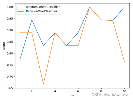
plt.plot(range(1,6),cross_clf,label='DecisionTreeClassifier')
plt.plot(range(1,6),cross_rf,label='RandomForestClassifier')
plt.xlabel('cv')
plt.ylabel('score')
plt.legend()
plt.show()
 
#随机森林的重要属性：estimators_,查看森林中树的情况
print(rf.estimators_)
for i in range(len(rf.estimators_)):
    print(rf.estimators_[i].random_state)
 
################换一种写法##############
cv = 10
for model in [RandomForestClassifier(n_estimators=5,random_state=42),DecisionTreeClassifier(random_state=42)]:
    cross = cross_val_score(model, wine.data, wine.target, cv=cv)
    plt.plot(range(1,cv+1),cross,label='{}'.format(str(model).split('(')[0]))
    plt.xlabel('cv')
    plt.ylabel('score')
    plt.legend()
plt.show()
 
##################学习曲线################
# superpa = []
# for i in range(200):
#     rf = RandomForestClassifier(random_state=42,n_estimators=i+1)
#     sc = cross_val_score(rf,wine.data,wine.target,cv=10).mean()
#     superpa.append(sc)
# plt.plot(range(1,201),superpa)
# print(max(superpa),superpa.index((max(superpa))))
# plt.show()
 
import numpy as np
from scipy.special import  comb
# 建立25棵树，当且仅当有13棵以上的树判断错误时，随机森林才会报错
# 如果一棵树的准确率在0.85上下浮动，那20棵树以上判断错误的概率
sum = np.array([comb(25,i)*(0.2**i)*((1-0.2)**(25-i)) for i in range(13,26)]).sum()
print(sum)

 

 

随机森林回归器

这里其实不用再多做介绍，与决策树回归一致，请回看这里。https://blog.csdn.net/weixin_44904136/article/details/126201929https://blog.csdn.net/weixin_44904136/article/details/126201929不过，值得一说的是它的应用，我们可以通过随机森林回归器填补缺失值。

测试集与训练集的划分思想：

xtrain：特征不缺失的值对应其他的n-1个特征 + 本来的标签

ytrain：特征不缺失的值

xtest：特征缺失的值对应其他的n-1个特征 + 本来的标签

ytest:特征缺失的值

适用于某一个特征大量缺失，而其他特征相对完整。

对，相对完整，也就是其他特征也可能存在缺失，那该怎么办呢？

答：我们首先通过检查特征空值，转化为布尔值加和（比较直观，0说明空，非0说明非空），进行排序，目的是先计算特征缺失少的部分，然后循环遍历。

选定特征之后，将其他特征的缺失值赋为0（这里注意复制原矩阵到新矩阵，避免原矩阵被补0覆盖），之后就是回归问题了。

案例代码

from sklearn.ensemble import RandomForestRegressor
import numpy as np
import matplotlib.pyplot as plt
from sklearn.model_selection import train_test_split
from sklearn.model_selection import cross_val_score
from sklearn.datasets import load_boston
import pandas as pd
from sklearn.impute import SimpleImputer  #填补缺失值
 
#评估指标
import sklearn
# print(sklearn.metrics.SCORERS.keys())
# sklearn.impute.SimpleImputer
boston = load_boston()
# print(boston.data.shape)  #(506, 13)
# print(boston.target)
 
#####################将数据集改为有缺失的数据集(特征为空)#####################
x_full,y_full = boston.data,boston.target
n_samples = x_full.shape[0]
n_features = x_full.shape[1]
 
rng = np.random.RandomState(0)
missing_rate = 0.5
n_missing_samples = int(np.floor(n_samples * n_features * missing_rate))  #np.floor向下取整
 
#所有数据要随机遍布在数据集的各行各列当中，而一个缺失的数据会需要一个行索引和一个列索引
# 如果能创造一个数组，包含3289个分布在0-506中间的行索引，和3289个分布在0-13之间的列索引
# 那我们就可以利用索引来为数据中的任意3289个位置赋空值
# 然后我们用0，均值和随机森林来填写这些缺失值，然后查看回归的结果
miss_features = rng.randint(0,n_features,n_missing_samples)
# randint(下限，上限，n) 请在下限和上限之间取出n个整数
 
miss_samples = rng.randint(0,n_samples,n_missing_samples)
# rng.choice(n_samples,n_missing_samples,replace=False) 抽取不重复的随机数
 
x_missing= x_full.copy()
y_missing = y_full.copy()
x_missing[miss_samples,miss_features] = np.nan
x_missing = pd.DataFrame(x_missing)
print(x_missing)
print('==============')
####################填补缺失值############################
####使用均值进行填补
imp_mean = SimpleImputer(missing_values=np.nan,strategy='mean') #实例化
x_missing_mean = imp_mean.fit_transform(x_missing)  #训练加导出
####使用0进行填补
imp_0 = SimpleImputer(missing_values=np.nan,strategy='constant',fill_value=0)
x_missing_0 = imp_0.fit_transform(x_missing)
 
#查看是否填补完毕
a = pd.DataFrame(x_missing_mean).isnull().sum()
b = pd.DataFrame(x_missing_0).isnull().sum()
# print(a)
# print(b)
 
####使用随机森林去填写缺失值
x_missing_reg = x_missing.copy()
#找出特征集中，缺失值从小到大排列的特征顺序（找索引）
sortindex = np.argsort(x_missing_reg.isnull().sum(axis=0)).values   #有索引 而sort()无索引
for i in sortindex:
    #构建新矩阵，防止下一步补0操作将原矩阵覆盖
    df = x_missing_reg
    fillc = df.iloc[:,i]
    df = pd.concat([df.iloc[:,df.columns != i],pd.DataFrame(y_full)],axis=1)
    #在新特征矩阵中，对缺失列补0,
    df_0 = SimpleImputer(missing_values=np.nan,strategy='constant',fill_value=0).fit_transform(df)
    #划分训练集和测试集
    ytrain = fillc[fillc.notnull()]  #被选中特征中存在值的行
    ytest = fillc[fillc.isnull()]    #被选中特征中空值的行
    xtrain = df_0[ytrain.index,:]
    xtest = df_0[ytest.index,:]
    #用随机森林预测特征
    rf = RandomForestRegressor(n_estimators=100,random_state=42)
    rf.fit(xtrain,ytrain)
    prediction = rf.predict(xtest)
    #将预测出的特征值填入缺失列中
    x_missing_reg.loc[x_missing_reg.iloc[:,i].isnull(),i] = prediction
print(pd.DataFrame(df))
print(x_missing_reg.isnull().sum())  #是否为空：是1 不是0，最后结果都为0，所以此时矩阵无空处，填补完成
 
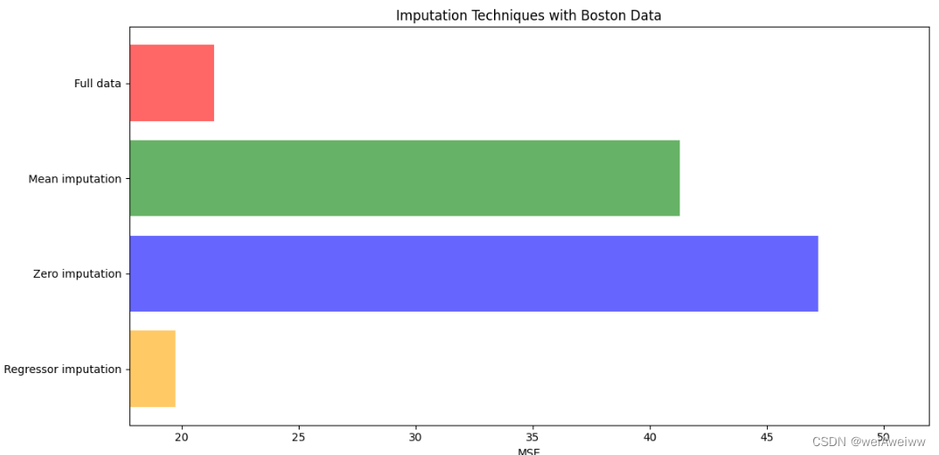
#################对填充好的数据进行模型训练###################
x = [x_full,x_missing_mean,x_missing_0,x_missing_reg]
mse = []
for i in x:
    estimator = RandomForestRegressor(n_estimators=100,random_state=42)
    estimator.fit(i,y_full)
    scores = cross_val_score(estimator,i,y_full,scoring='neg_mean_squared_error',cv = 5).mean()
    mse.append(scores * -1)
 
# print(mse) #mse越小越好
print([*zip(['x_full','x_missing_mean','x_missing_0','x_missing_reg'],mse)])
 
#################绘图################################
x_labels = ['Full data','Mean imputation','Zero imputation','Regressor imputation']
colors = ['r','g','b','orange']
plt.figure(figsize=(12,6)) #画出画布
ax = plt.subplot(111)   #添加子图
 
for i in np.arange(len(mse)):
    ax.barh(i,mse[i],color=colors[i],alpha=0.6,align='center')  #横向条形图
ax.set_title('Imputation Techniques with Boston Data')
ax.set_xlim(left=np.min(mse)*0.9,
            right=np.max(mse)*1.1) #刻度
ax.set_yticks(np.arange(len(mse)))
ax.set_xlabel('MSE') #x轴名字
ax.invert_yaxis()
ax.set_yticklabels(x_labels)
plt.show()

 

 

随机森林的介绍就到此结束喽，但是对于性能的提升问题，也就是调参问题，我们下一篇来接着说~