基于opencv、matlab的多十字靶标的自动识别 与 模板匹配多次匹配的问题_opencv 十字型 匹配

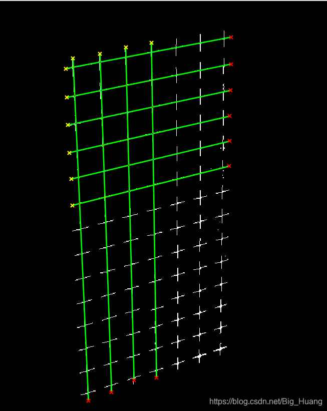
       相机标定时常会使用标定板进行标定，常用的标定法有张正友老师的平板标定，常用的标定板有棋盘标定板和圆盘标定板，但是很多地方使用TSAI两步标定法时会使用自制的标定靶标吗，例如我们采用的按规则排序的十字靶标，拍摄得到的实物如下：

方法一:  Hough 直线检测求交点

      为了得到各十字中心的坐标，常用的方法为使用hough直线检测，得到横竖的所有直线的表达式并通过交点解算来得到交点的坐标，这一块我也做了，但是事实来看，需要多次试探得到合适的阈值等参数，也就是说程序的泛化性比较差，这应该也是我代码写的不好，但是实在找不到好的方法，因为阈值参数的选取确实是得调整的，而且同一标定板上下的明暗是会有差异的，后面我也是为了避免后面的点的获取，只选了前部分识别度较高的十字，但是因为是作为标定的输入，这么多点数已经够了。当然也可以微调参数得到所有的交点，但是我这个标定板有一个十字因为制作时打错了，所以我人为滤掉这一行；下面是我使用MATLAB给出的方法：

front = imread('a.bmp');
back = imread('a_back.bmp');
%img = imread('cali.bmp');
img = front - back;
img_gray = rgb2gray(img);
 
%%  获取行
thresh = graythresh(img_gray);
B = im2bw(img_gray, thresh);
B = bwmorph(B, 'skel', 1);    % 骨架提取
B = bwmorph(B, 'spur', 2);    % 去毛刺
[H, theta, rho] = hough(B, 'Theta', 30:0.03:89);
peaks = houghpeaks(H, 14);
rows = houghlines(B, theta, rho, peaks);
imshow(B), hold on;
temp = [];
row_line = [];
for k = 1:length(rows)
    temp = [temp; rows(k).point1];
end
[temp, I] = sort(temp, 1, 'ASCEND');
for k = 1 : 6    % 希望的行数
    xy = [rows(I(k, 2)).point1, rows(I(k, 2)).point2];
    plot([xy(1,1), xy(1, 3)], [xy(1,2), xy(1,4)], 'LineWidth', 2, 'Color', 'green');%画出线段
    plot(xy(1,1), xy(1,2), 'x', 'LineWidth', 2, 'Color', 'yellow');%起点
    plot(xy(1,3), xy(1,4), 'x', 'LineWidth', 2, 'Color', 'red');%终点
    row_line = [row_line; xy];  %[startX startY endX endY]
end
 
%%    获取列
thresh = graythresh(img_gray);
B = im2bw(img_gray, thresh);
%B = bwmorph(B, 'skel', 1);    % 骨架提取
%B = bwmorph(B, 'spur', 1);    % 去毛刺
[H, theta, rho] = hough(B, 'Theta',-30:0.03:30);
peaks = houghpeaks(H, 7);
columns = houghlines(B, theta, rho, peaks);
%imshow(B), 
hold on;
temp = [];
column_line = [];
for k = 1:length(columns)
    temp = [temp; columns(k).point1];
end
[temp, I] = sort(temp, 1, 'ASCEND');
for k = 1 : 4    % 希望的列数
    xy = [columns(I(k, 1)).point1, columns(I(k, 1)).point2];
    plot([xy(1,1), xy(1, 3)],[xy(1,2), xy(1,4)],'LineWidth',2,'Color','green');%画出线段
    plot(xy(1,1),xy(1,2),'x','LineWidth',2,'Color','yellow');%起点
    plot(xy(1,3),xy(1,4),'x','LineWidth',2,'Color','red');%终点
    column_line = [column_line; xy];  %[startX startY endX endY]
end
 
%%  获取交点像素坐标
intersection = [];
line = [row_line; column_line];
for i = 1 : length(line) - 1
    p1 = line(i, :); 
    k1 = (p1(2) - p1(4)) / (p1(1) - p1(3));
    b1 = p1(2) - k1*p1(1);
    for j = i+1 : length(line)
        p2 = line(j, :);
        k2 = (p2(2)-p2(4))/(p2(1)-p2(3));
        b2 = p2(2)-k2*p2(1);
          %求两直线交点
        x = -(b1-b2) / (k1-k2);             
        y = -(-b2*k1+b1*k2) / (k1-k2);
          %判断交点是否在两线段上  可能存在斜率十分相近导致上式分母接近零而误解
        if min(p1(1),p1(3)) <= x && x <= max(p1(1),p1(3)) && ...
           min(p1(2),p1(4)) <= y && y <= max(p1(2),p1(4)) && ...
           min(p2(1),p2(3)) <= x && x <= max(p2(1),p2(3)) && ...
           min(p2(2),p2(4)) <= y && y <= max(p2(2),p2(4))    
            plot(x,y,'.');
            intersection = [intersection; [x, y]];  %依次第一至最后行 与 第一至最后列
        end
        
    end
end

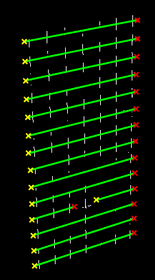
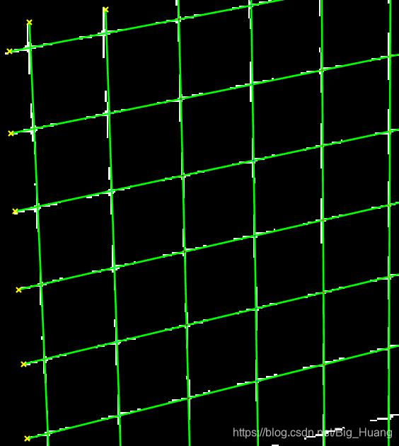
得到的结果如下：

   分别为所有行、所有列；设置的六行四列的交点，对应交点其实已经求出，并在四图中标出（红点）

方法二:   OpenCV 轮廓查找和模板匹配

使用OpenCV对图像进行处理，经过简单处理后，先进行轮廓查找找到所有的十字轮廓，其中很可能混入因阈值不当引入的噪点的轮廓，但是我们可以使用轮廓面积来约束，找到适中大小的轮廓，其实就是某个十字靶标的图案，将此作为模板来对对象进行查找，考虑会出现多次查找的问题，就是对某一轮廓稍微左右移动得到的轮廓依旧匹配度较高，因此会被识别为模板，但是又不能提高识别度，识别度要求一旦提高则会丢失很多不是很请清楚的目标，故在稍微降低识别度的情况下（此时肯定存在重复识别的问题），比较两轮廓的相对距离来剔除重复识别的对象，主要是先将所有相近的目标全部赋值为第一个目标（此处可能略粗糙，也是误差产生的地方）。然后剔除相同的目标，在对所得所有点按照空间实际顺序进行排列以便对应实际的世界坐标（标定的时候需要）；代码如下：

import numpy as np
import cv2
import os
 
 
GREEN = (0, 255, 0)
RED = (0,0,255)
filename = 'pixelCoordinate.txt'
 
# **** Basic processing of the original image and extract all contours ****
img = cv2.imread('cali.bmp')
imgray = cv2.cvtColor(img,cv2.COLOR_BGR2GRAY)
ret,thresh = cv2.threshold(imgray,30,255,0)
image, contours, hierarchy = cv2.findContours(thresh, cv2.RETR_TREE,cv2.CHAIN_APPROX_SIMPLE)
             
# ***********  Find an appropriate contour for the template   **********              
for cnt in contours:
        if cv2.contourArea(cnt) > 120:
                (x,y,w,h) = cv2.boundingRect(cnt)
                template=imgray[y:y+h, x:x+w] 
                rootdir=("C:/Users/Administrator/Desktop/cali/")
                if not os.path.isdir(rootdir):
                        os.makedirs(rootdir)
                cv2.imwrite( rootdir + "template.bmp",template)
                break
        
# ************ Find all matched contours ************
w, h = template.shape[::-1]                    
res = cv2.matchTemplate(imgray, template, cv2.TM_CCOEFF_NORMED)
threshold = 0.75
 
point = []
point_temp = []
loc = np.where(res >= threshold)
for pt in zip(*loc[::-1]):
        point.append([pt[0], pt[1]])     
length = len(point)
print(' Before Processing:    ' + str(length))
 
# **** Assign the corresponding point of a similar template to one of them ******
i = 0
while(i < length):
        for j in range(i + 1, length):
                if ( np.abs(point[j][0] - point[i][0]) < 4 and np.abs(point[j][1] - point[i][1]) < 4):
                        point[j] = point[i]
        i = i + 1
 
# ***************** Eliminate similarities  *******************
for i in point:
        if i not in point_temp:
                point_temp.append(i)        
print(' After Processing:    ' + str(len(point_temp)))
 
 
# ********** In order from left to right, from top to bottom ***********
point_temp.sort(key = lambda x:x[0])
for i in range(0, 92, 14):
        point_temp[i : i+14].sort(key = lambda x:x[1])
 
 
# ***************** Display and save the results **********************
if os.path.exists(filename):
        os.remove(filename)
for index in range(len(point_temp)):
        cv2.rectangle(img, tuple(point_temp[index]), (point_temp[index][0] + w, point_temp[index][1] + h), RED, 1)
        x = int(point_temp[index][0] + w/2)
        y = int(point_temp[index][1] + h/2)
        with open(filename, 'a') as file:
                file.write(str(x) + '  ' + str(y) + "\n")
                cv2.circle(img, (x, y), 0, GREEN, 0)       
 
cv2.imshow('Result', img)
cv2.imwrite('Result.bmp', img)
 

结果如下：

总结:

       按照最后结果来看，方法一得到的精度更高，但是会人为调整较多参数，适应性差；方法二的精度没有第一个高，但是适应性比较强，这就比较尴尬，后面有需要会在精度方面做调整，毕竟这个方法还是比较简洁；

      各位有啥好的方案欢迎评论交流！！！